Plastics classification

Goal

In this tutorial, you will analyze the hyperspectral images of plastic samples. Your goal is to learn how to use Breeze to create a model based on machine learning which can be used for classification of different types of plastic.

The data

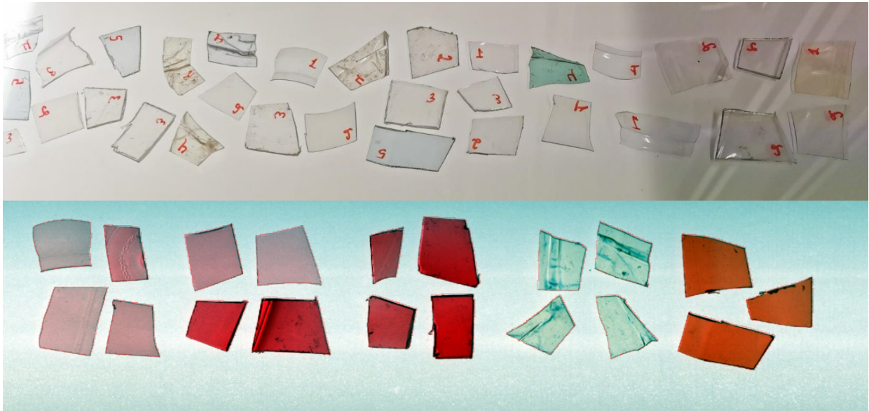
The data consist of two images containing samples of five different types of plastic.

• Polyethylene terephthalate bottle (PET BOTTLE)

• Polyethylene terephthalate sheet (PET SHEET)

• Polyethylene terephthalate glycol (PET G)

• Polyvinyl chloride (PVC)

• Polycarbonates (PC)

The tutorial images contain samples of known plastic type which will be used as training data set and test set. The spectral acquisition was carried out using a HySpex SWIR-384 camera, with a spectral range of 930 - 2500 nm. The plastic samples were placed on a moving stage and broadband halogen lamps were used as illumination sources. The data used in this tutorial is reduced using average binning, 2 times spatially and 4 times spectrally leaving the images with 192 pixels across the field of view, and 72 spectral bands. This was done to reduce the size of the data files for internet downloading.

In this tutorial you will learn how to:

1. Use Manual segmentation to use your mouse to select samples in an image that will be used as the training set.

2. Use Grid and Inset segmentation to add additional data points that will be used for the training.

3. Training of a Machine learning classification model.

4. Classification of the images using your machine learning model.

5. Add additional training data to your model and then re-train and apply it to your image.

6. Do a real-time analysis workflow with object segmentation and classification and apply it using the simulator camera.

Download tutorial image data

Start Breeze.

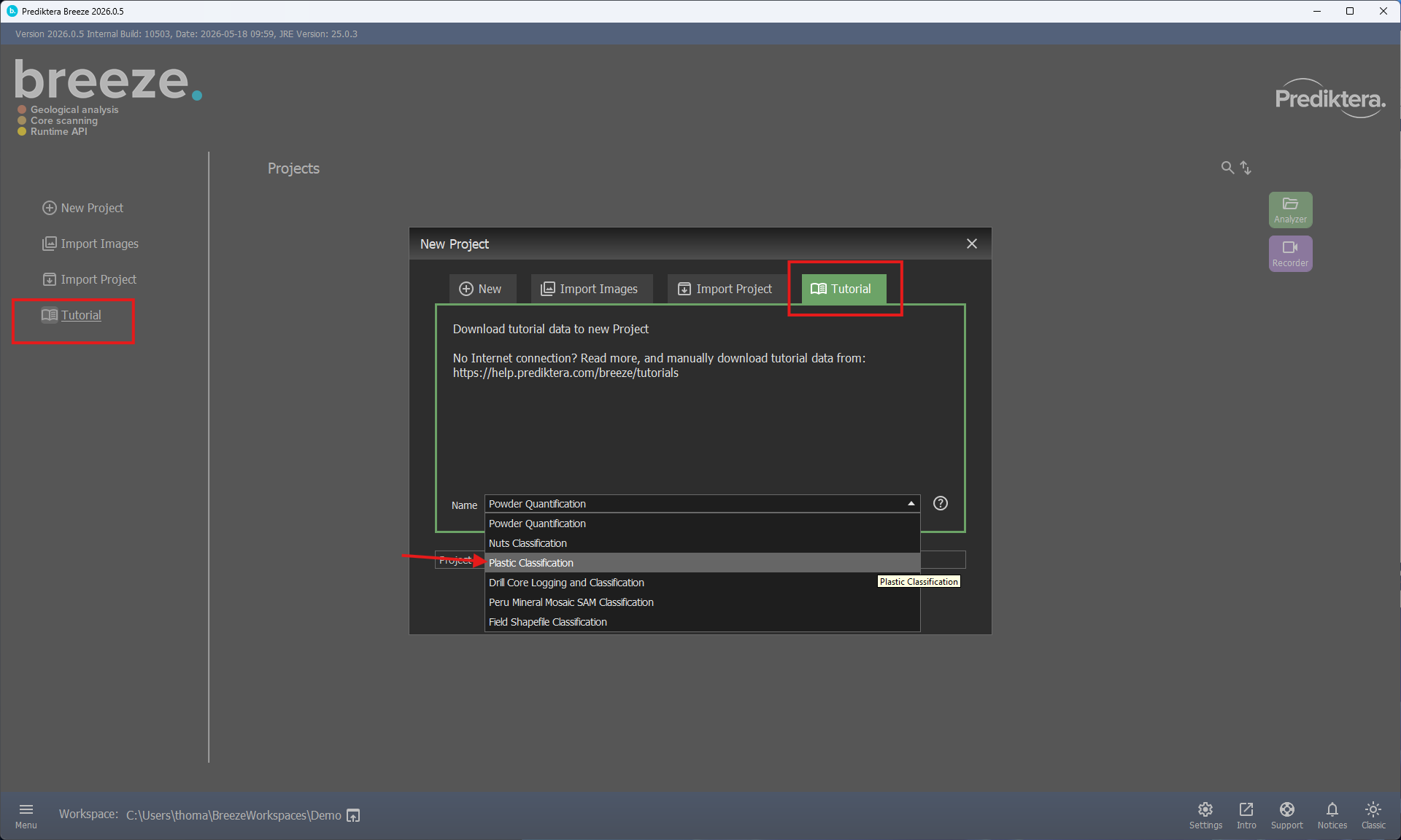
On the home screen, select Tutorial from the left side menu (Or select New Project and open the Tutorial tab).

Select “Plastic Classification” in the Name drop-down menu.

Click OK to start downloading the image data.

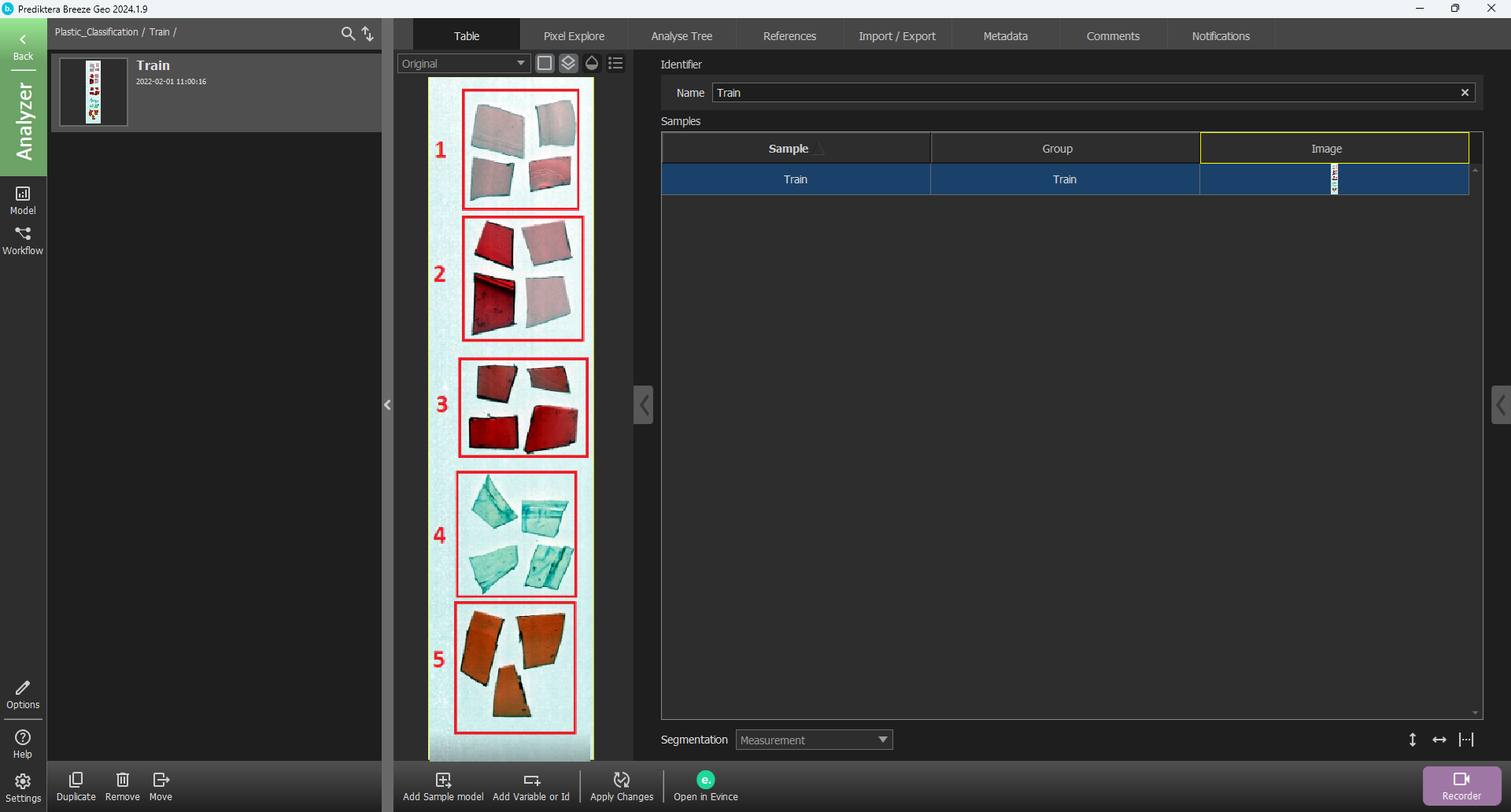
After the tutorial data is downloaded you will see the following table:

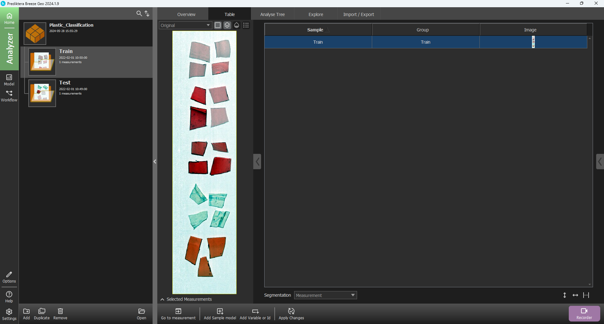
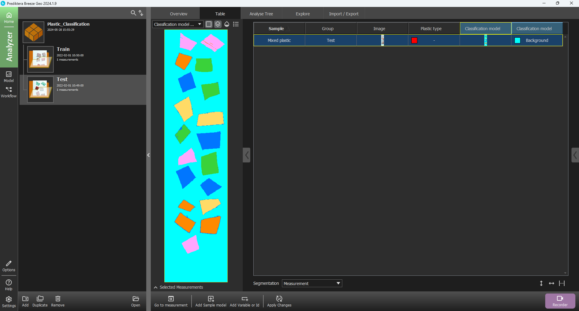
A project called “Plastic_Classification” has now been created. It includes one training image and one test image. You can click on a row in the table to see the preview image (pseudo-RGB) for each image.

The image data in the project is organized into two groups called Train and Test. Select the train group and click on the Open button to open it, or double-click on the group on the left. You can also select Go to measurement to open the group and show the measurement that is selected in the table.

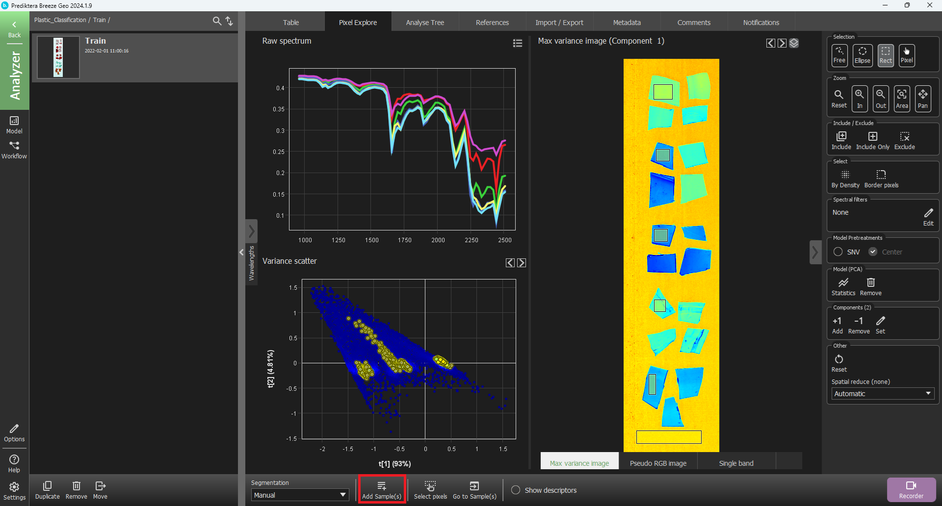
Click on the Pixel Explore tab.

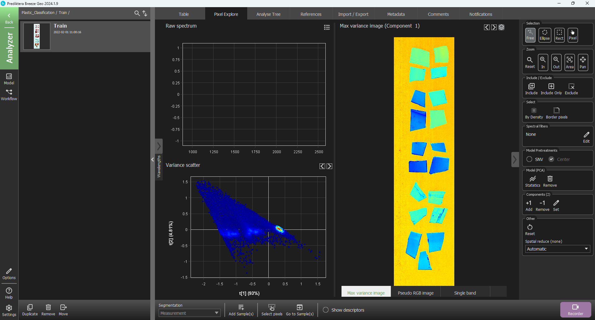
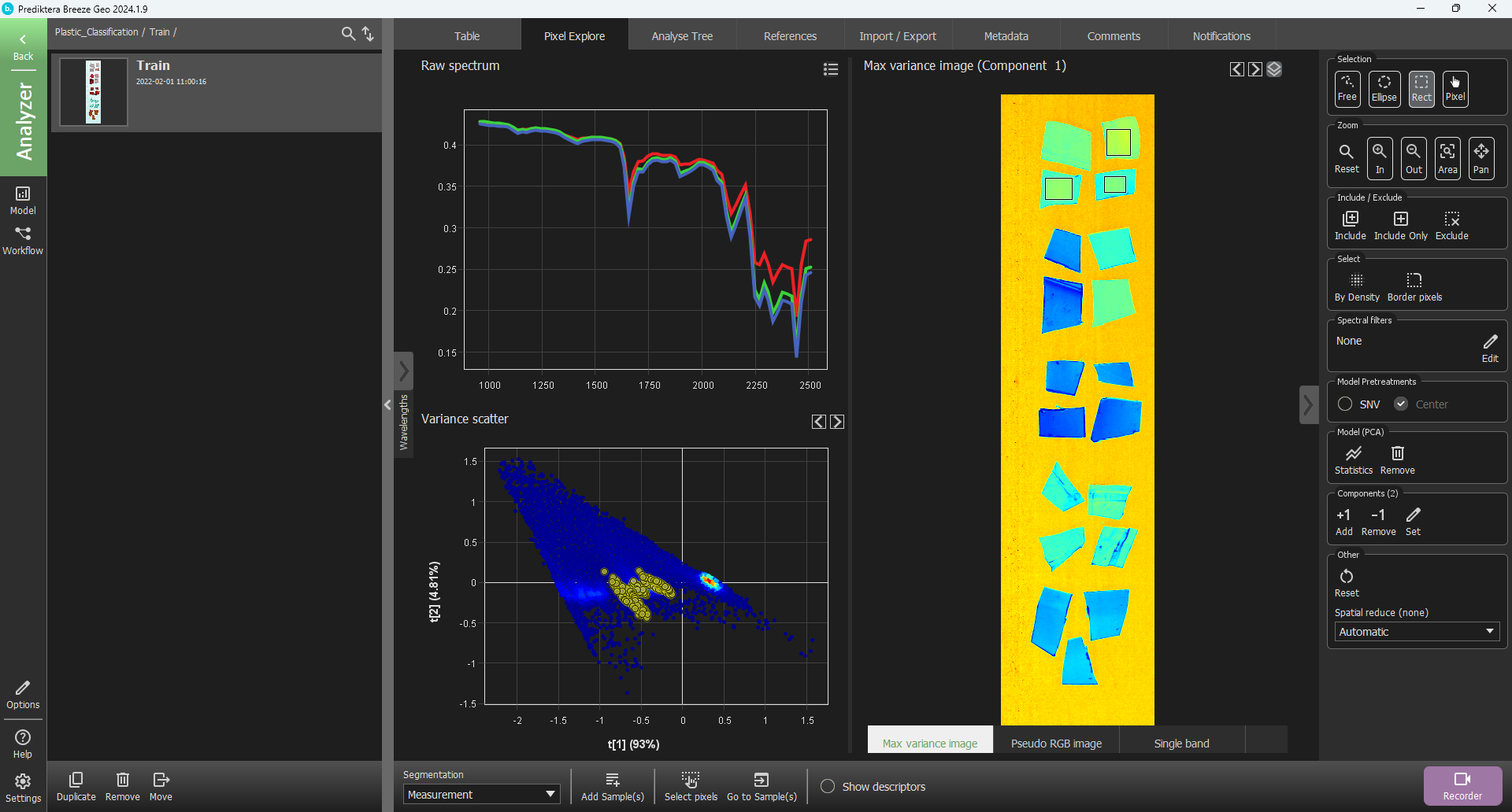
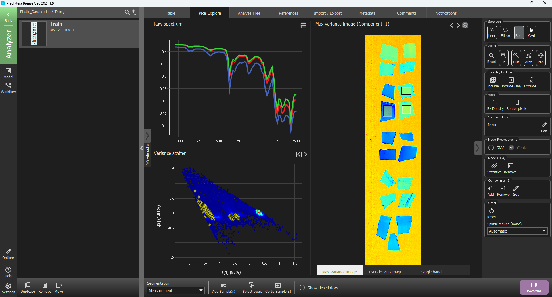
To do a quick analysis of the spectral variation in the image select Create in the menu on the right to create a PCA model based on all pixels in the image.

Each point in the Variance scatter plot corresponds to a pixel in the image. The points in the scatter plot are clustered based on spectral similarity. The color of the points in the scatter plot are based on density (i.e. red = many points close to each other).

The Max variance image is colored by the variation in the 1st component of the PCA model (the X-axis in the scatter plot, t1), and visualizes the biggest spectral variation in the image. In this case, this is the difference between the sample objects and the background.

Click and drag in the Variance scater plot to select of a cluster of points and see where those pixels are located in the image. Move the cursor around in the image to see the spectral profile for individual pixels or do a selection to see the average spectra for several pixels.

Select training data

The training data consists of five different types of plastic as mentioned previously.

1. PET Bottle

2. PET Sheet

3. PET G

4. PVC

5. PC

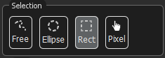
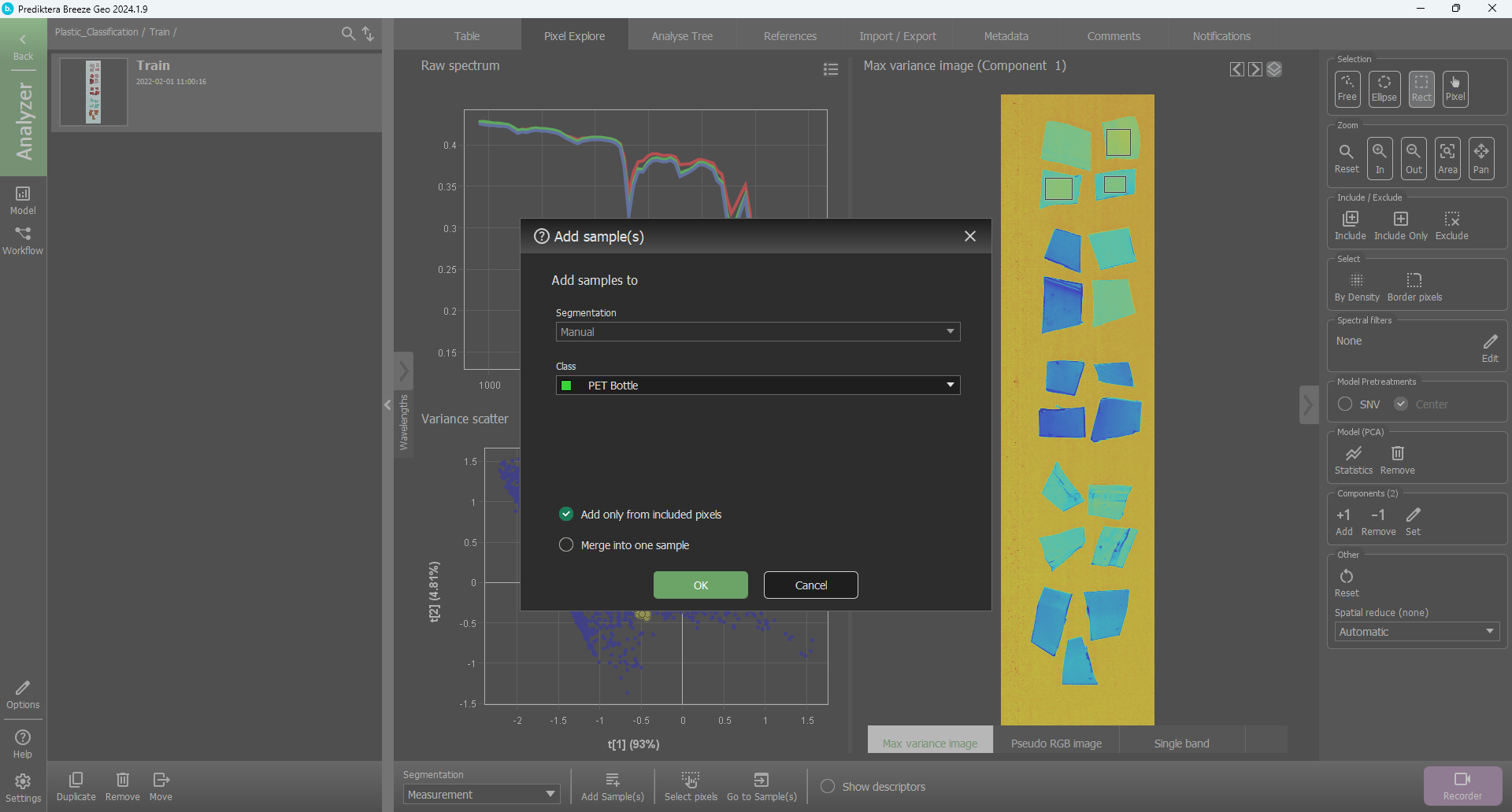
To acquire the data from each class needed to train the model you will manually select areas in Pixel Explore. Choose the Selection tool Rect that makes rectangular areas.

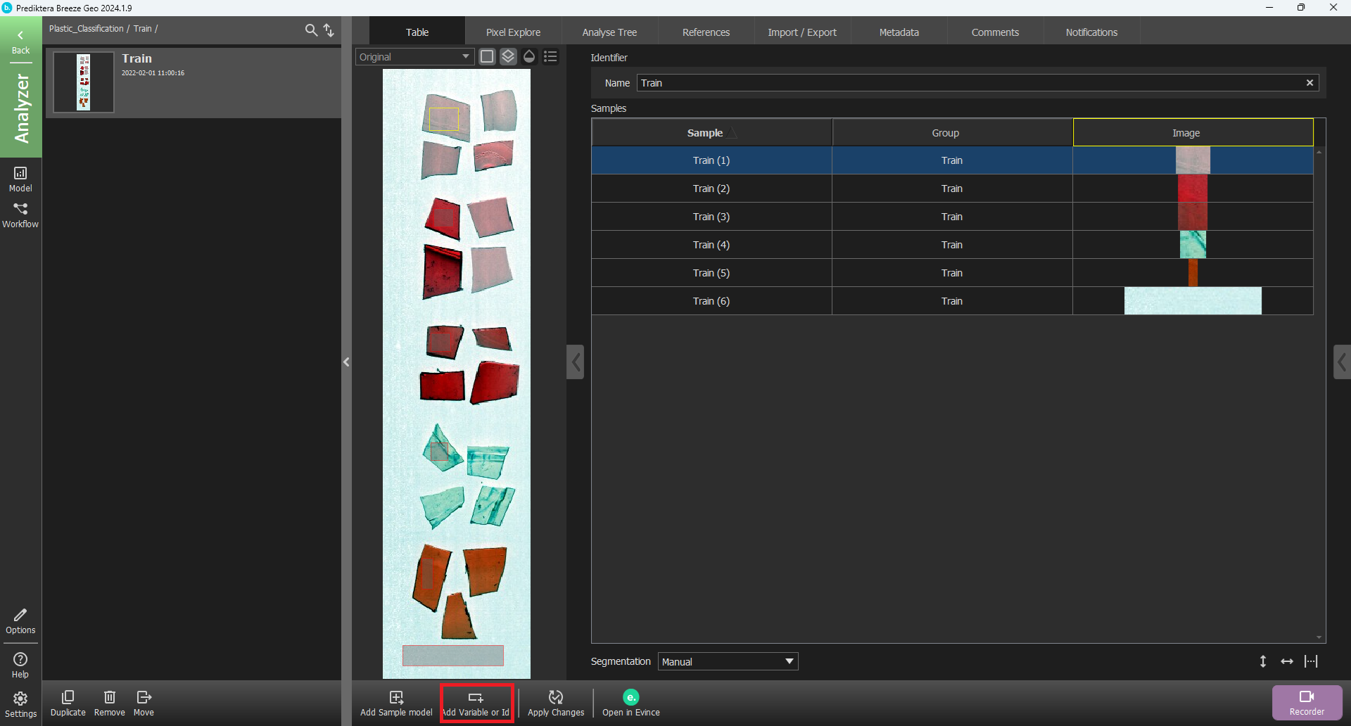
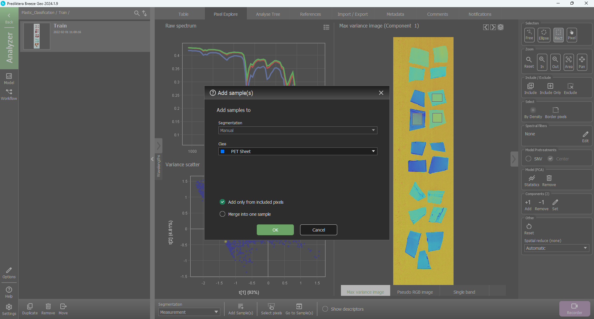
Now select areas in the Max variance image corresponding to the five different plastic types and the background. To select more than one area in the image hold down Ctrl on your keyboard. To zoom, use the scroll wheel on your mouse. To pan the zoomed image hold down the scroll wheel and move the image. First, select areas from five samples and the background. After you have selected the different samples and the background, click Add Sample(s) and then select OK.

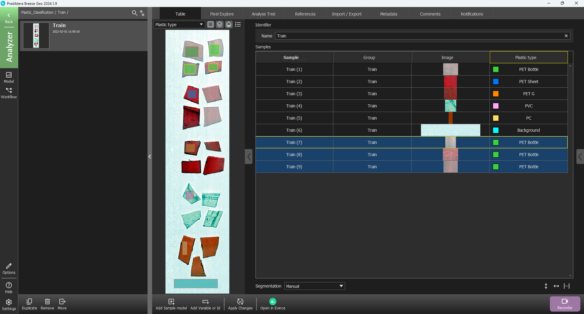
You will now be back in the Table view and you can see your six manually selected segmentations.

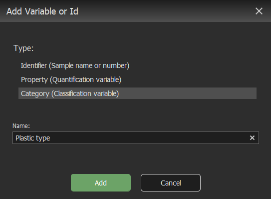
Now you need to enter the known class information for the training samples. First select Add Variable or Id.

Select Category (Classification variable).

Change the name to “Plastic type” and click Add.

A new column has appeared in the table.

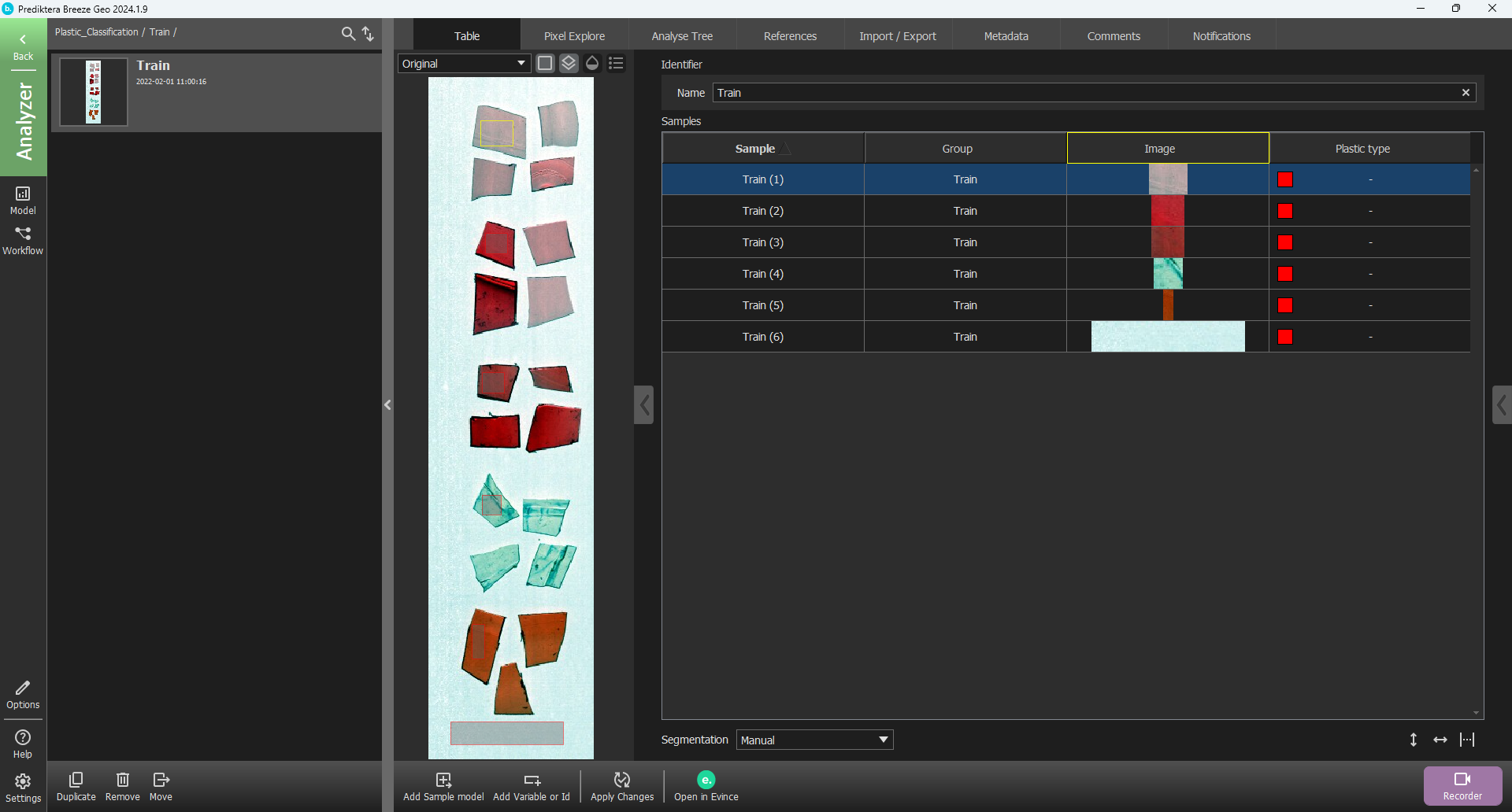
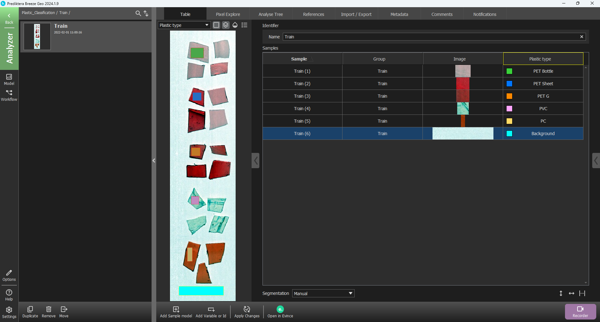
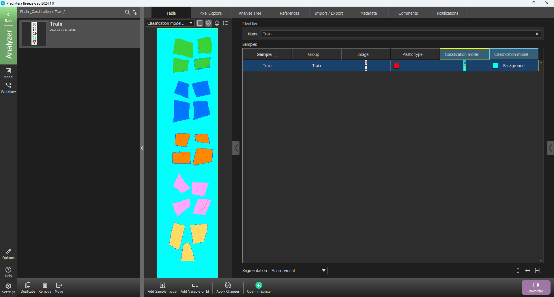
Right-click on a row in the new Plastic type column corresponding to the PET bottle sample, and under New class write “PET Bottle” and press Enter on your keyboard or click Add.

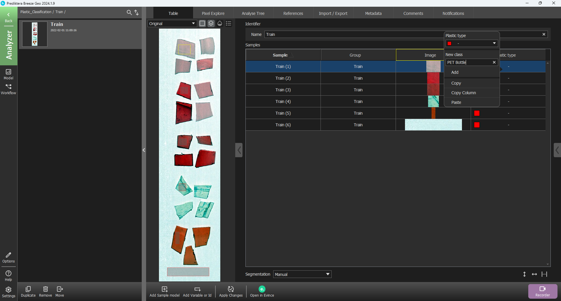
You will now see that the class of the first manual sample is PET Bottle. Do the same procedure to add the classes, “PET Sheet”, “PET G”, “PVC”, “PC” and “Background”. (Please note that the colors used for each class might be slightly different in the version of Breeze you are using).

Create a Machine learning model and then retrain it with more data

You will now create a Machine learning (ML) model based on the training set. But before going into the model wizard to create the model you need to apply a second layer of segmentation to get more training data for the ML model. In this tutorial, you will use the Grid and inset segmentation to do that.

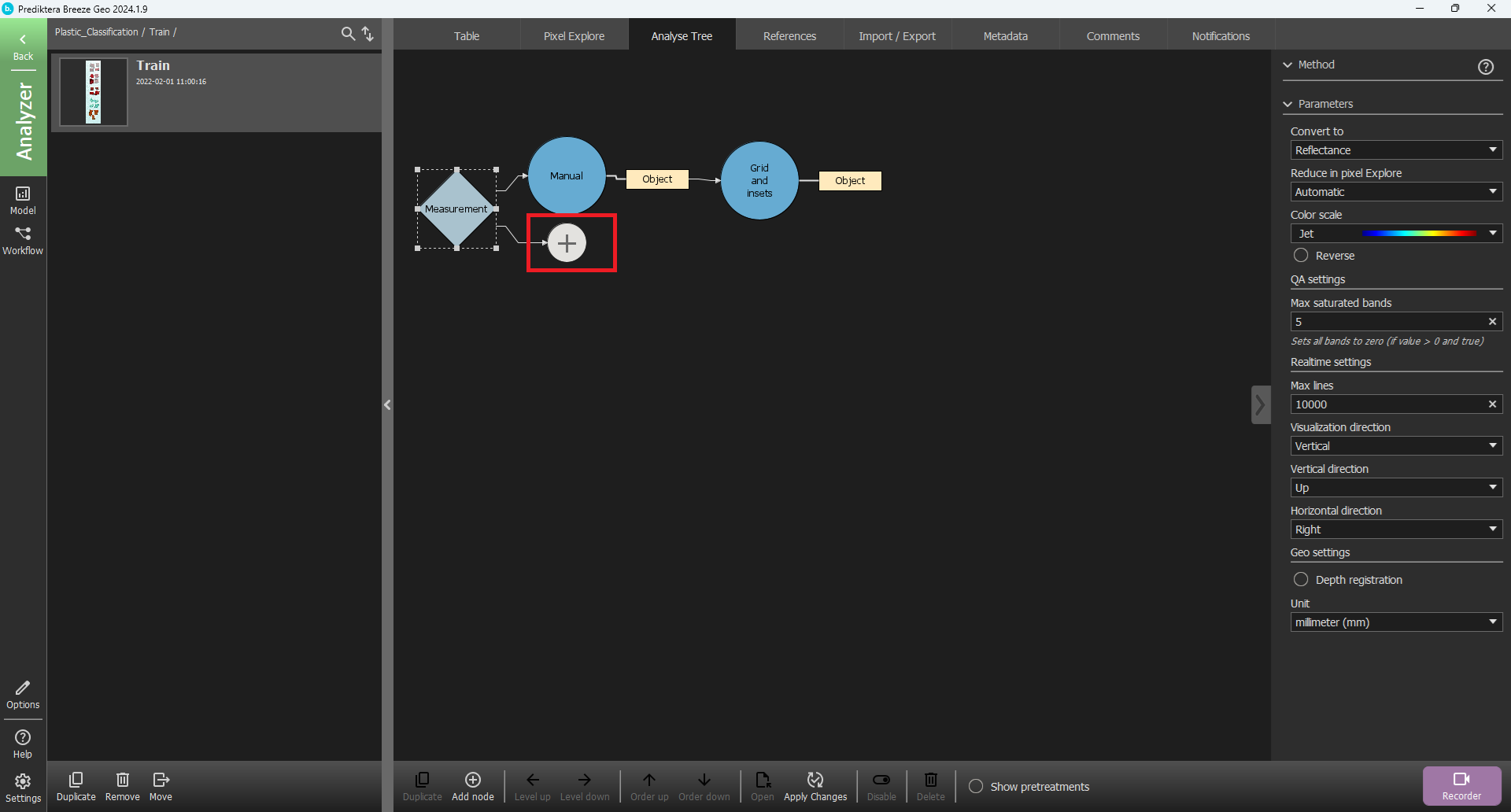
Go to the Analyse Tree tab.

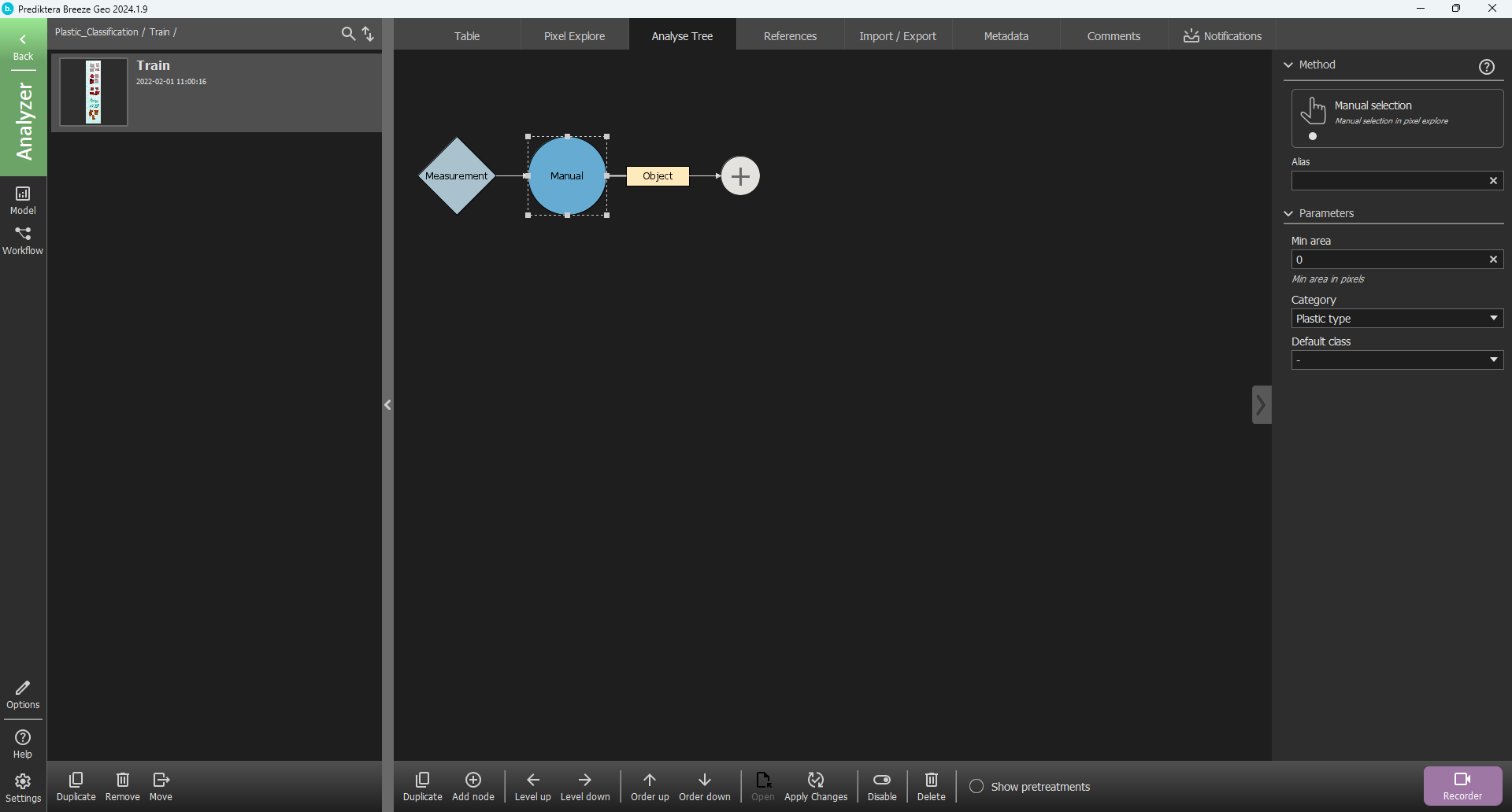
Click on Manual and you will see a plus sign appear.

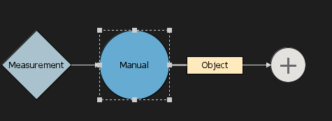
Click on the plus sign.

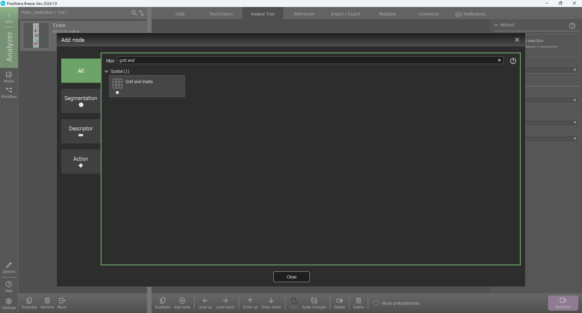
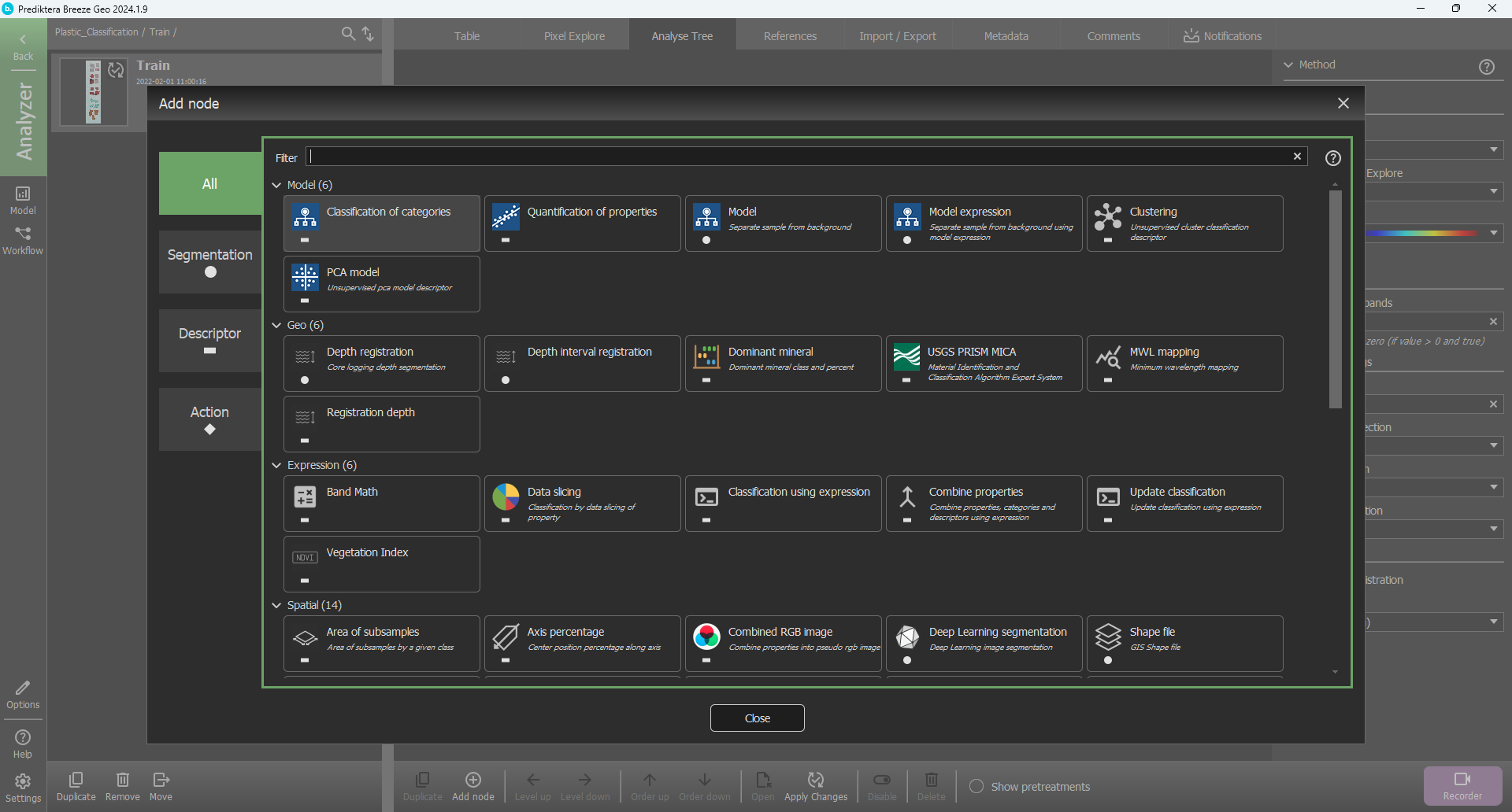
Select Segmentation, then select Grid and inset and click OK.

In the menu to the right, change the 3x3 under the Grid parameter to 6x6.

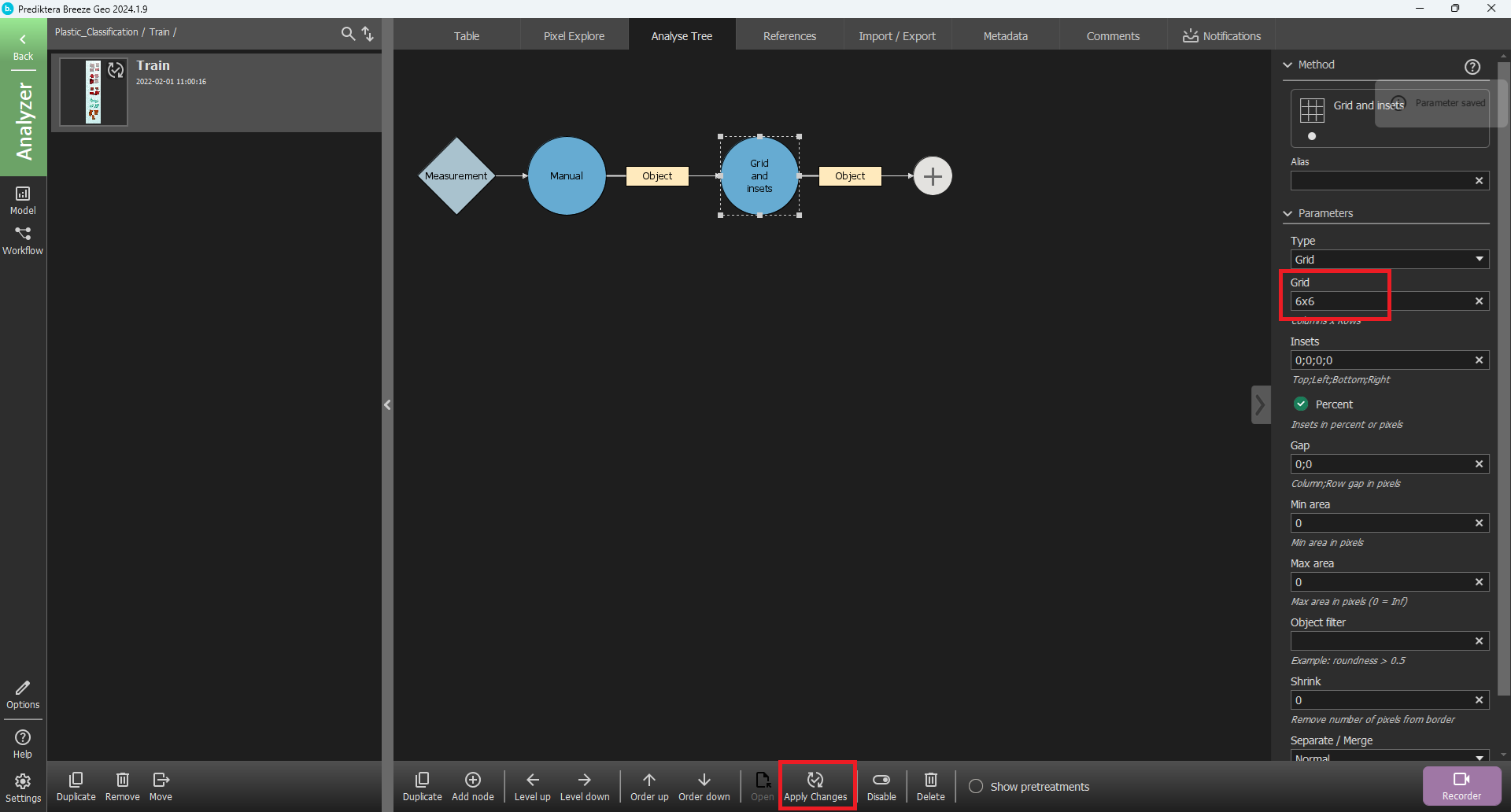
Select Apply Changes.

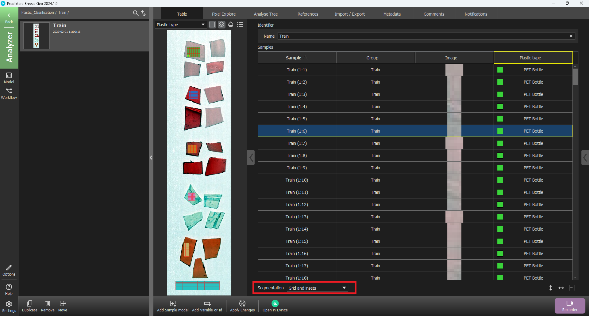
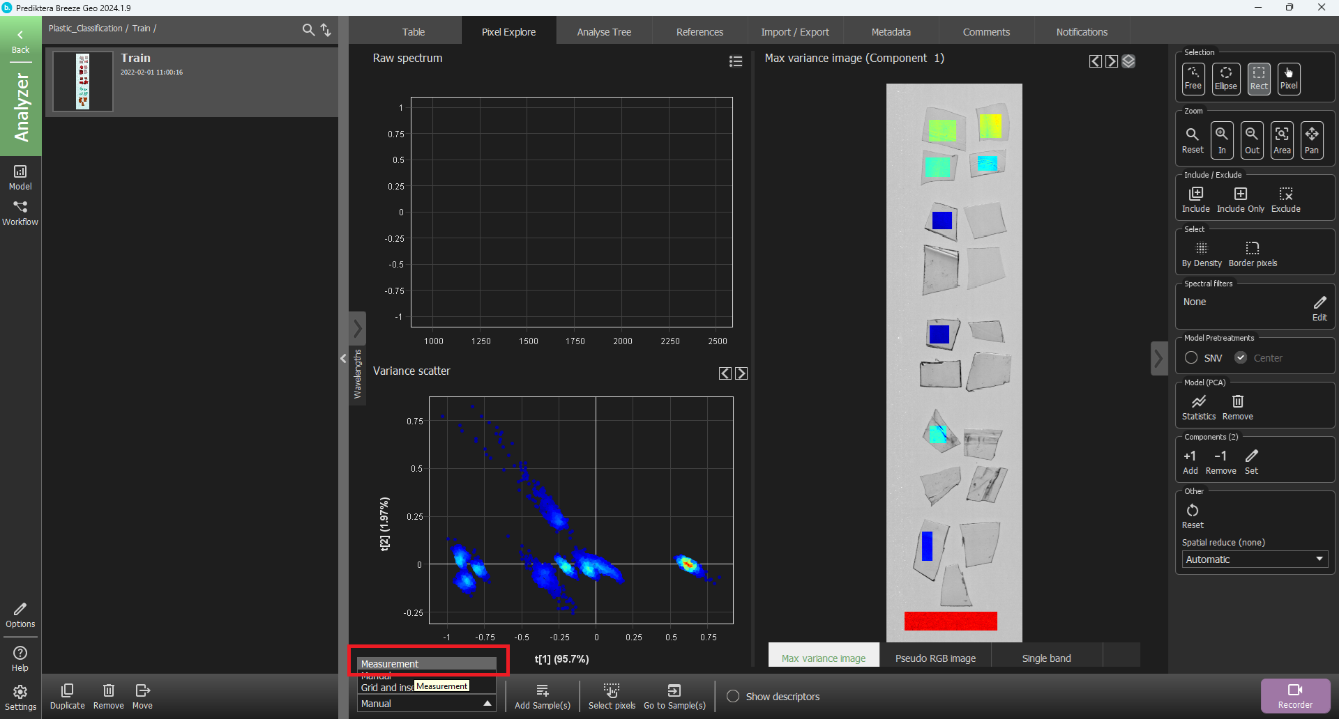
If you change the Segmentation in the drop-down menu under the Table to Grid and Inset you can see the 6x6 grid added under each manually selected area.

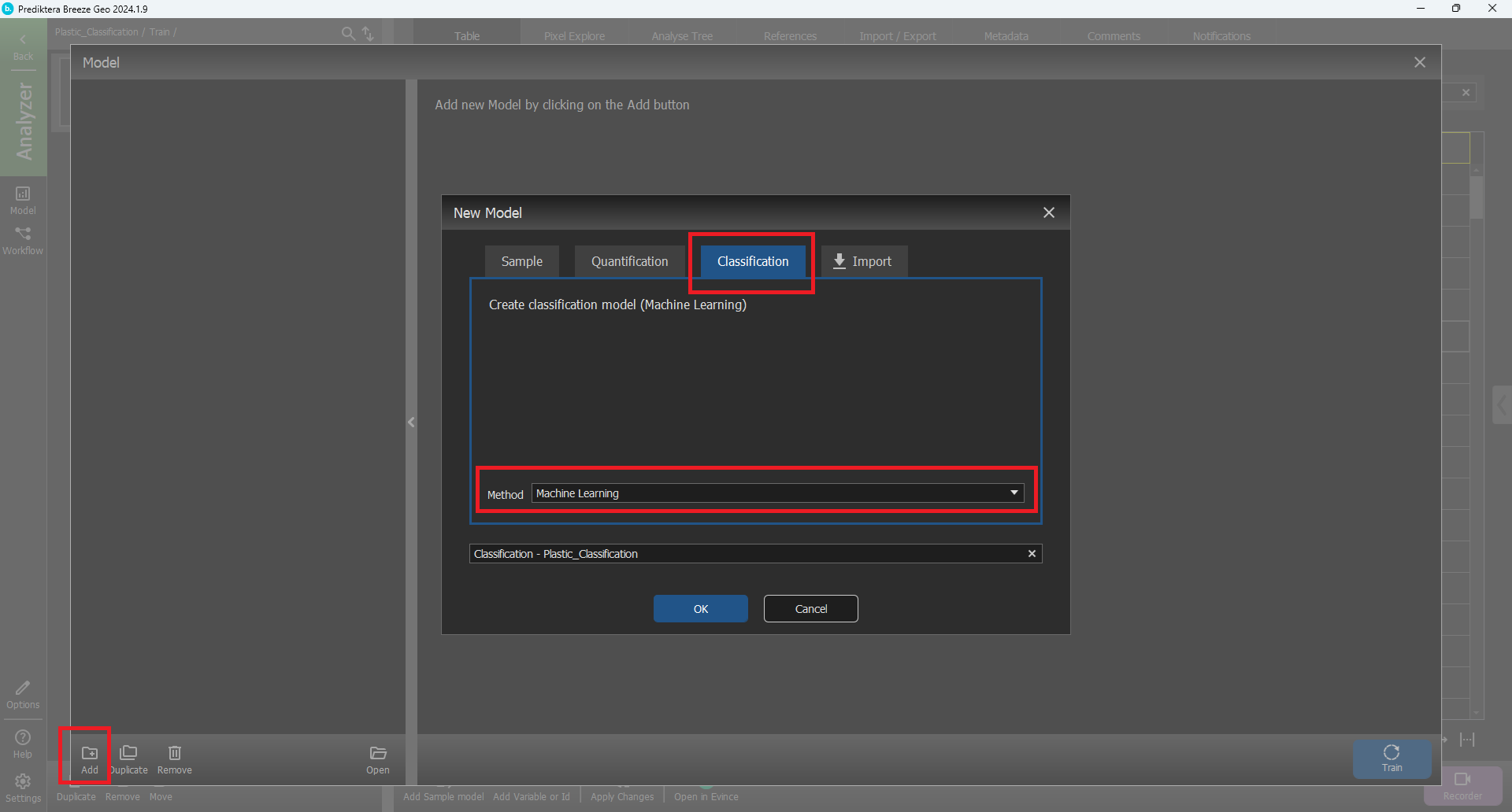
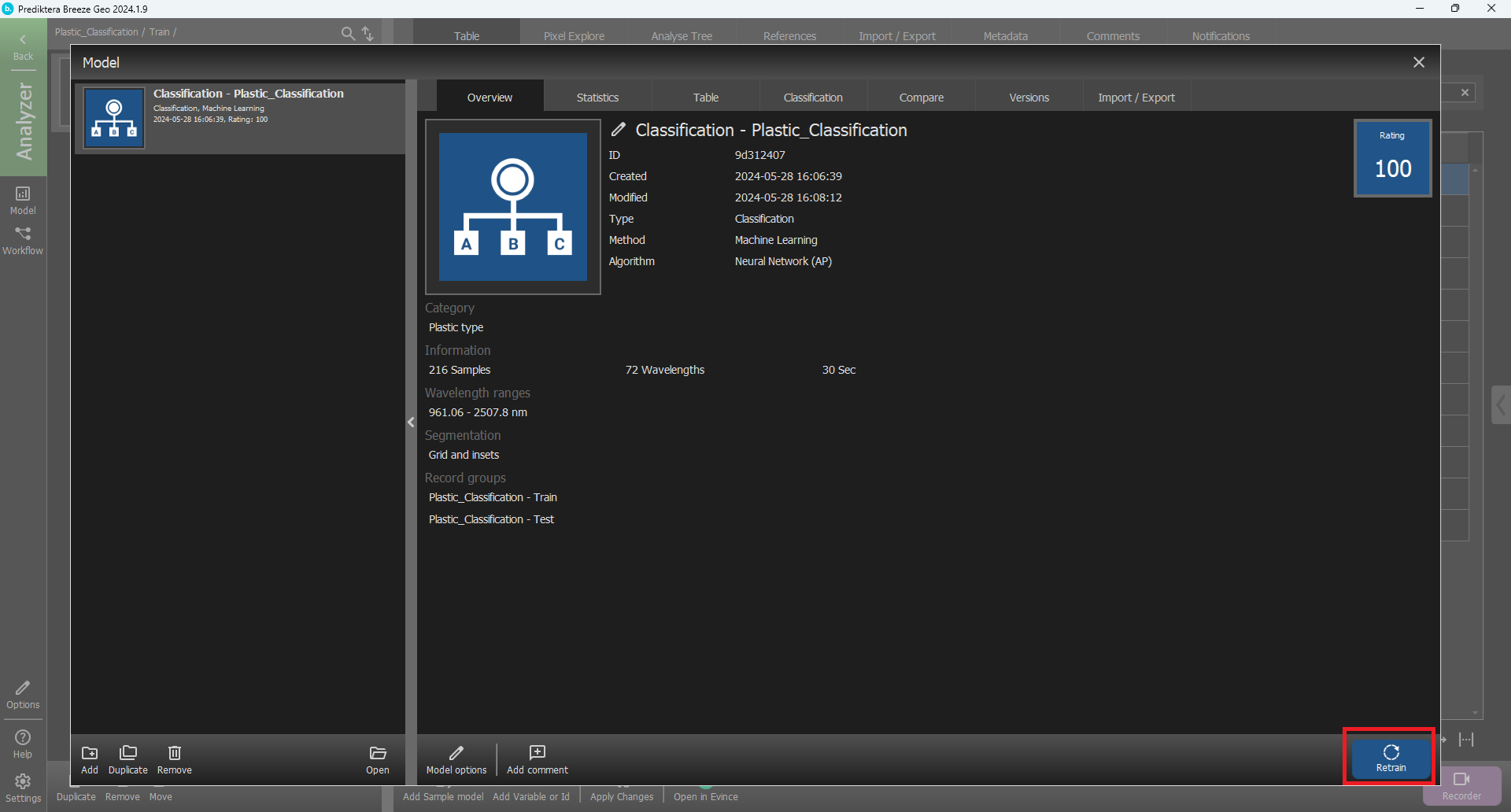
Select the Model button on the left side of the window.

In Model click the Add button in the bottom left corner.

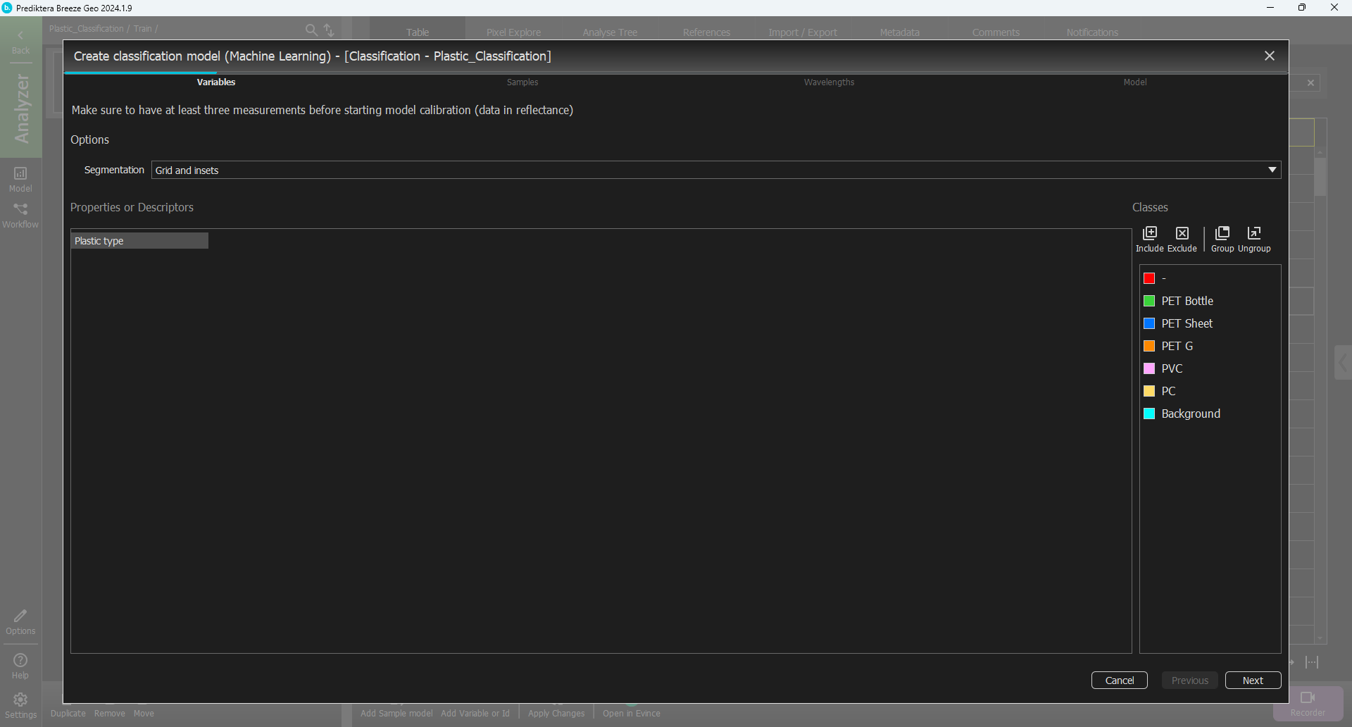
Select Classification, and in the menu select Machine Learning, and click OK (You can change the name on the model if you want).

In the first step of the Classification wizard, you can see that the “Grid and inset” segmentation is selected. and the Plastic type descriptor that you will use to build the model. Click Next.

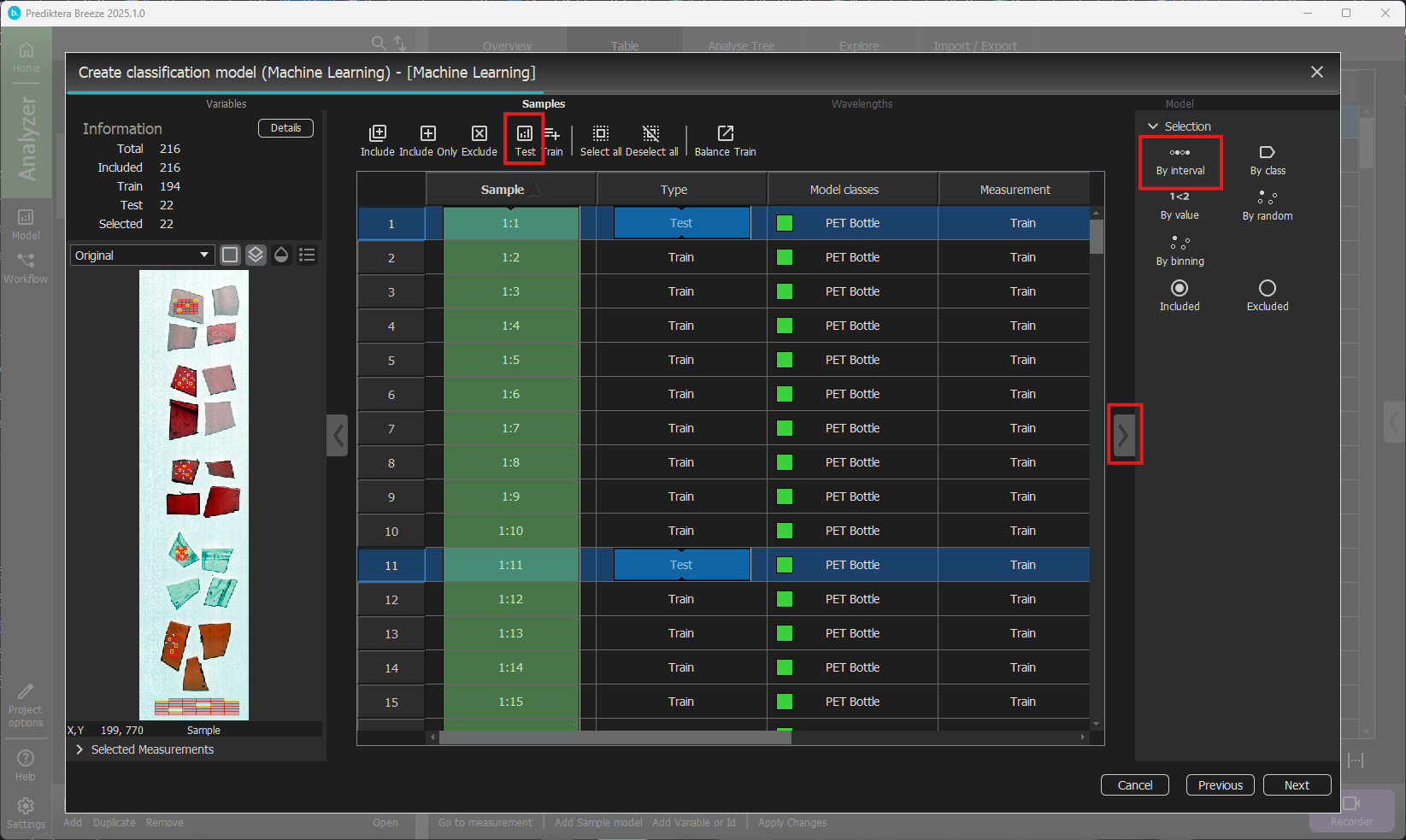
In the next step of the wizard, you can select the samples that you want to include in the model. By default, the measurements from the “Train” group have been included since they have entered class information. Each sample that will be used for the training corresponds to one of the segments in the 6x6 grid on the plastic pieces as you can see on the left in the following image.

Expand the panel to the right and select By interval. Start position and interval can be left at their defaults of 1 and 10. With the selected interval, click Test above the table to change type to Test.
Click Next.

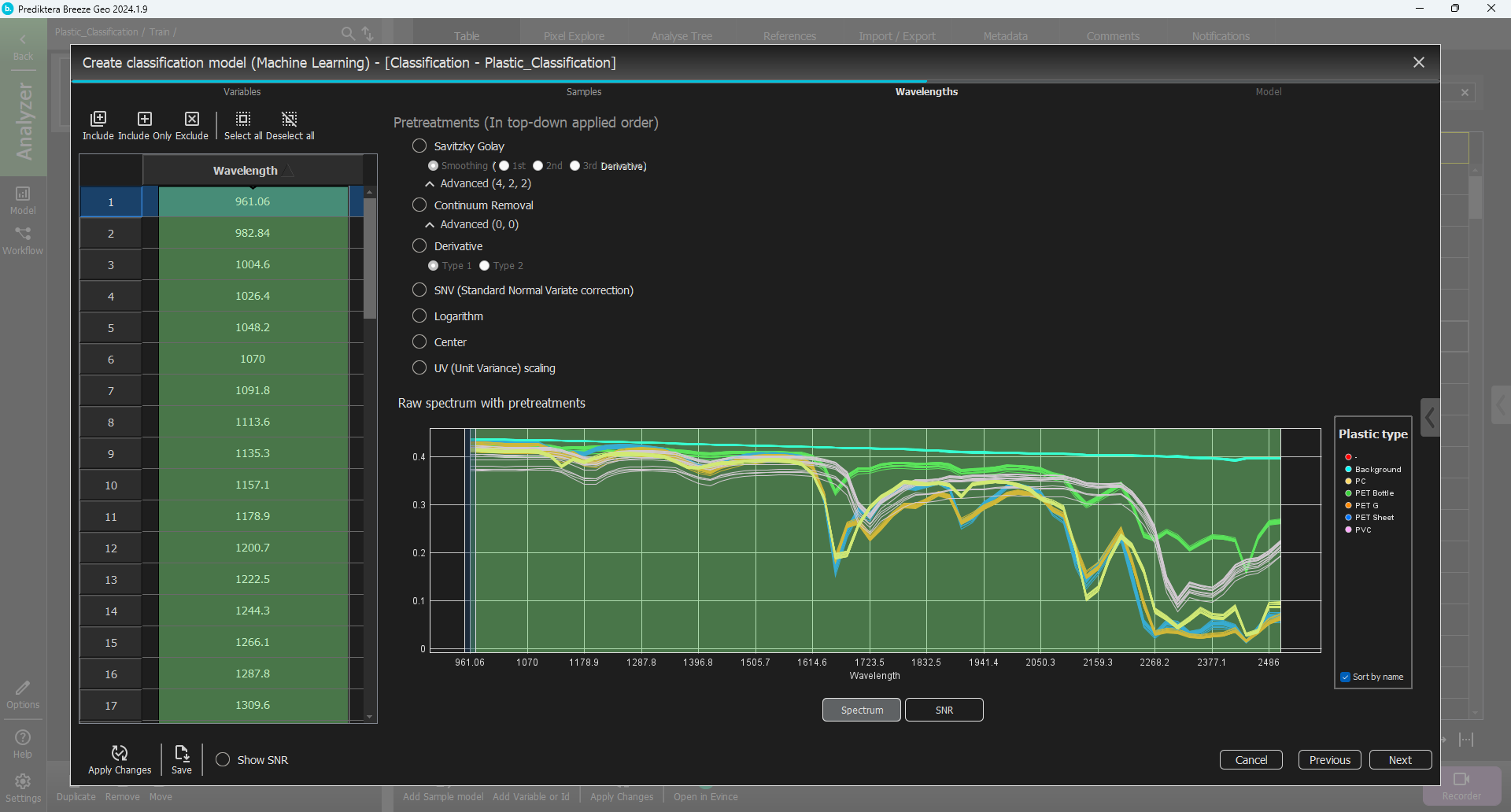
By default, all wavelength bands are included and no pretreatment is added. The graph on the right is showing the average spectrum for each sample (i.e. each grid). Above the graph, there is an option to select different Pretreatments for the spectral data. All default settings here are OK.
Click Next.

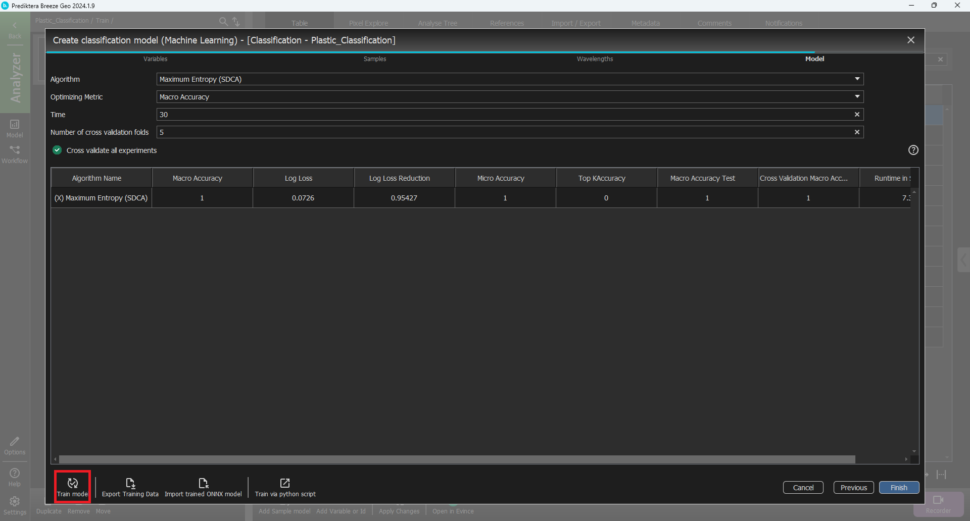
In the last step, we will train the model. For this tutorial, we will use Maximum entropy as the ML model. Open the Algorithm drop-down and scroll down until you find the Maximum Entropy (SDCA). The training time is good at 30 seconds.

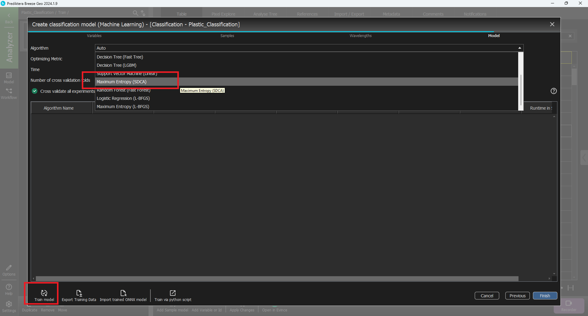
Select Train and wait for the training to finish.

You now have a trained model.

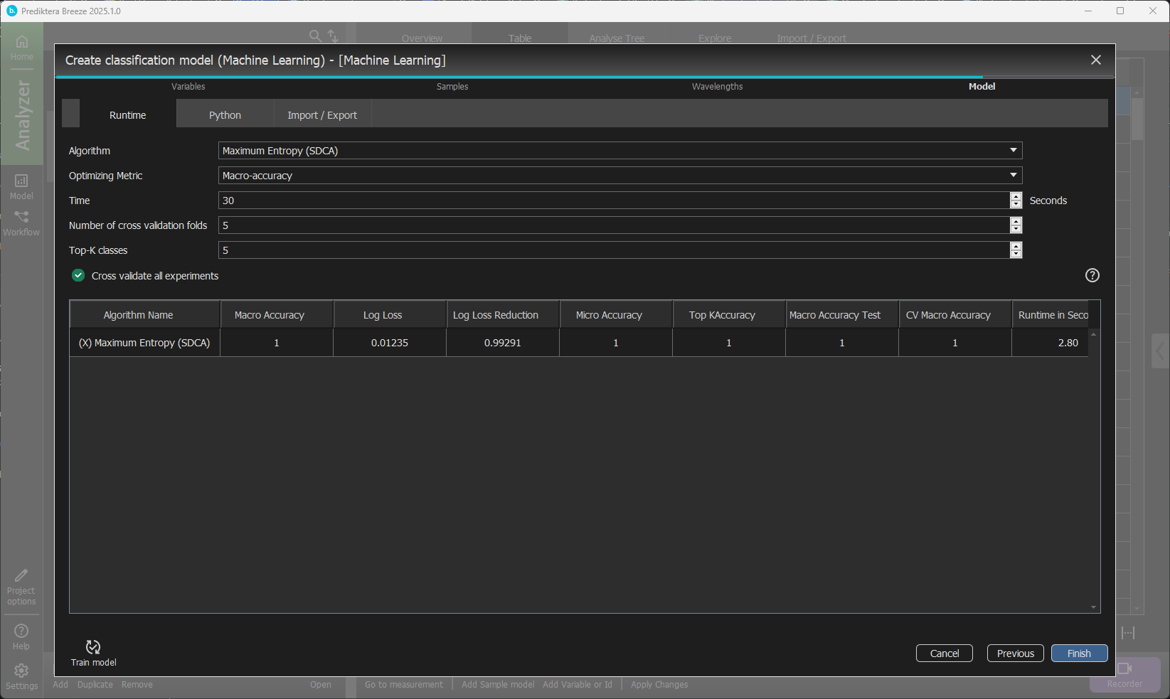
Click Finish.

Go to the Classification tab to see how well the trained model worked on the training set.

Close the model dialog, select the Train group and go to the Analyse Tree.

Click on Measurement and select the plus sign.

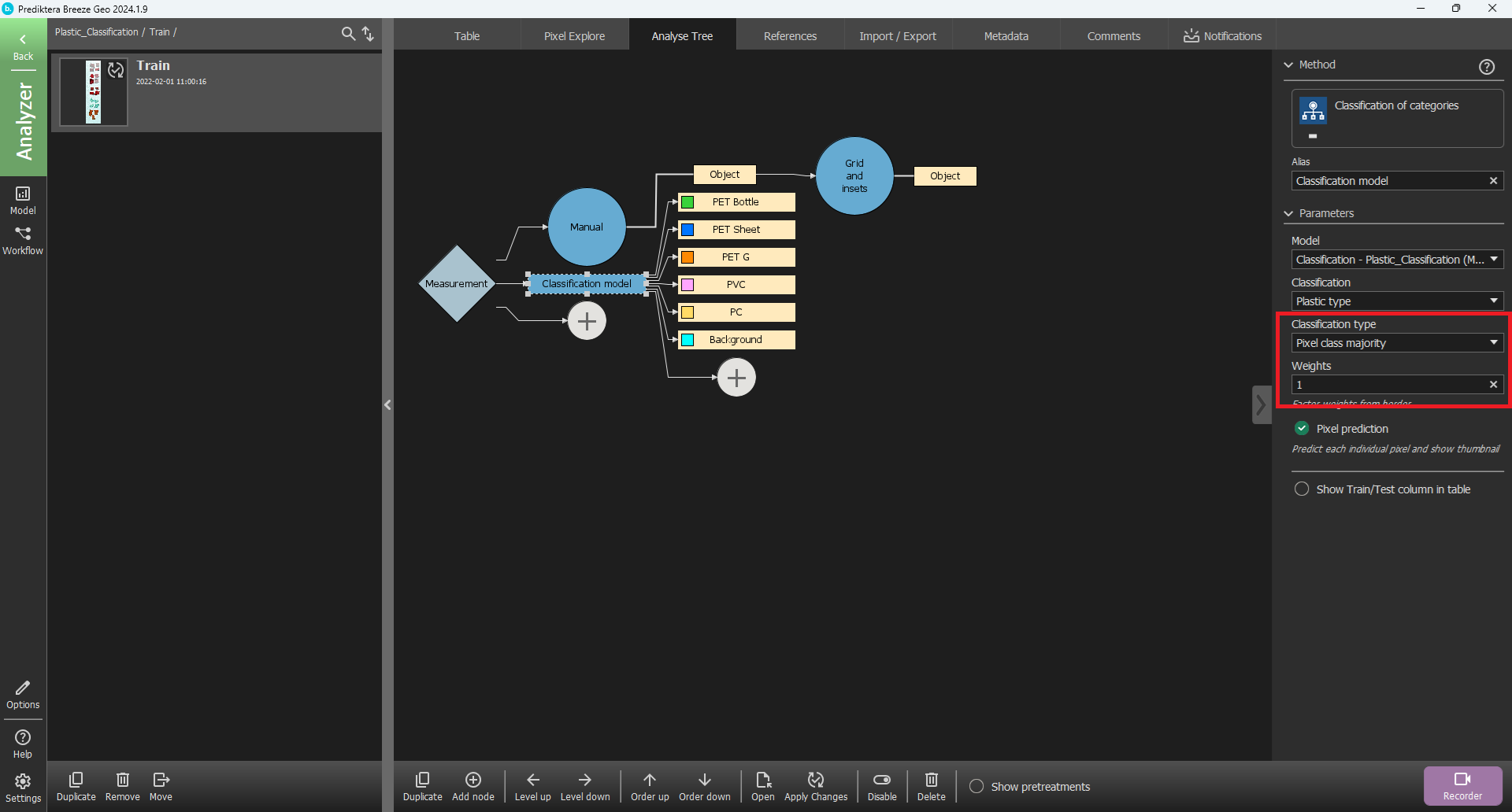
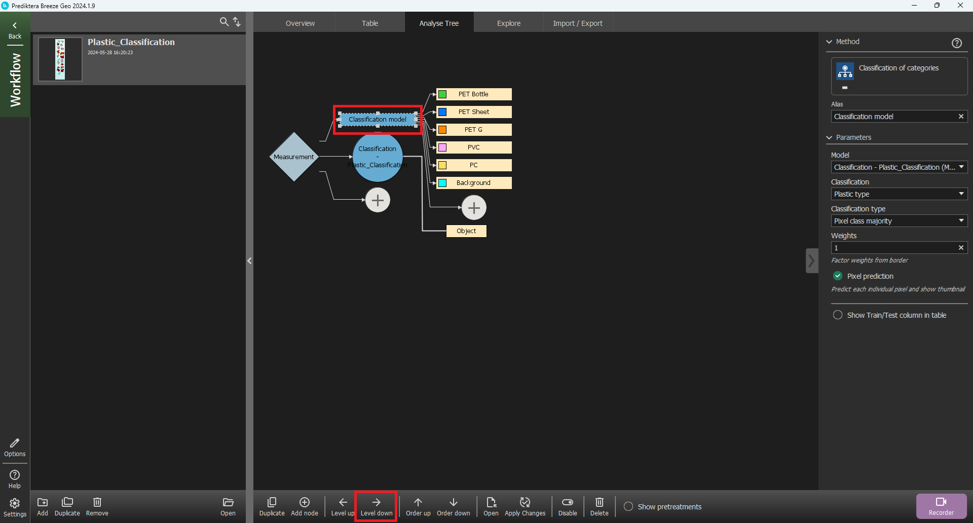
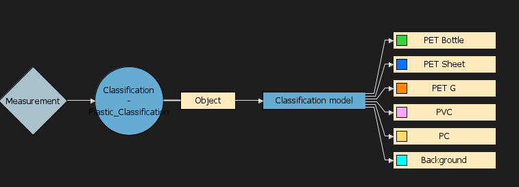
Select Descriptor, choose Classification of categories and write an Alias to identify it, for example: “Classification model”.

The classification model will now be added to the Analysis tree. In the menu on the right, set the Classification Type to Pixel class majority. The Weights field should have value 1.

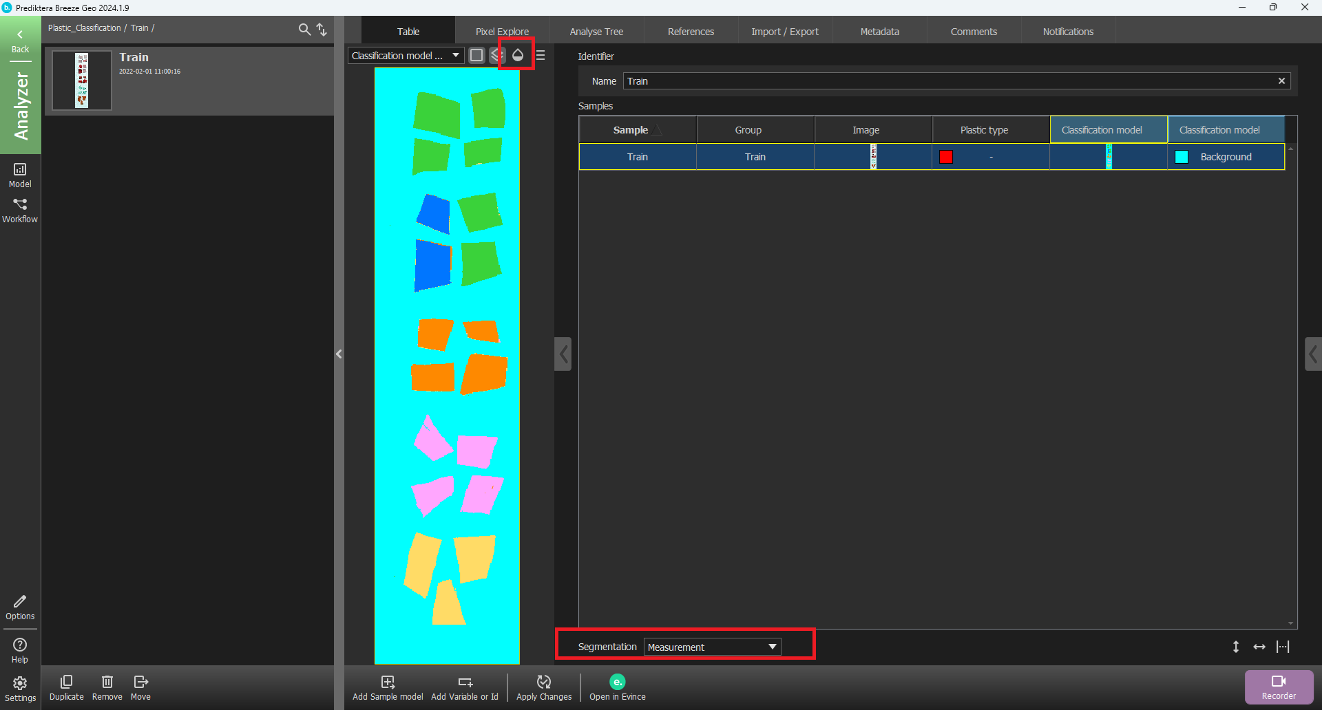
Go to the Table view again and select Apply changes. The classification model will now be applied to your image. Select the Measurement segmentation level and click on the image in the column for the classification model to see the results in the image. You can also select the button above the image to add a legend showing the color coding for the classes.

The distinction between samples may be clearer by deselecting the Blend button, shaped like a drop, located above the image.

As you can see, in this case, two of the “PET Sheet” samples are wrongly classified as “PET Bottle”. To see if these can be correctly classified, we will add more of them to the training data.

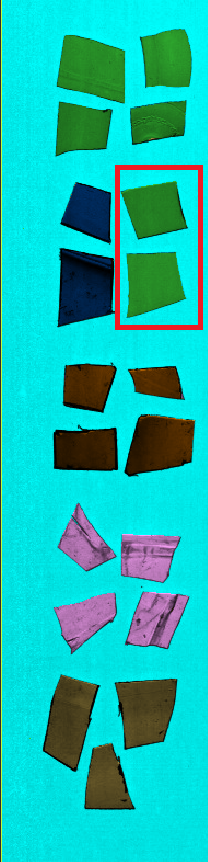
Since these two classes seem to be a bit difficult to distinguish we will add the rest of the plastic bits for both of them to the training of the model.

Go to Pixel Explore and select an area in each of the three unused PET Bottle samples (hold down ctrl and select with the mouse).

Then select Add Sample(s) and select the “PET Bottle” class.

If you go to the Table you can see that this area has now been added to the Manual segmentation.

Go back into pixel explore.

As you can see the view looks different. This is because we are on the manual segment level. We can change this by opening the drop-down menu labelled Segmentation and changing the selection to Measurement.

Now select the three pieces of the PET Sheet.

Select Add Sample(s), select “PET Sheet” as your class, and click OK.

Go back to the Model view and click Retrain on the model we created earlier.

In step 1 click Next.

In Step 2 you need to add the new segments that you created. As you can see in under Information there are segments 432 in total but only 216 are included.

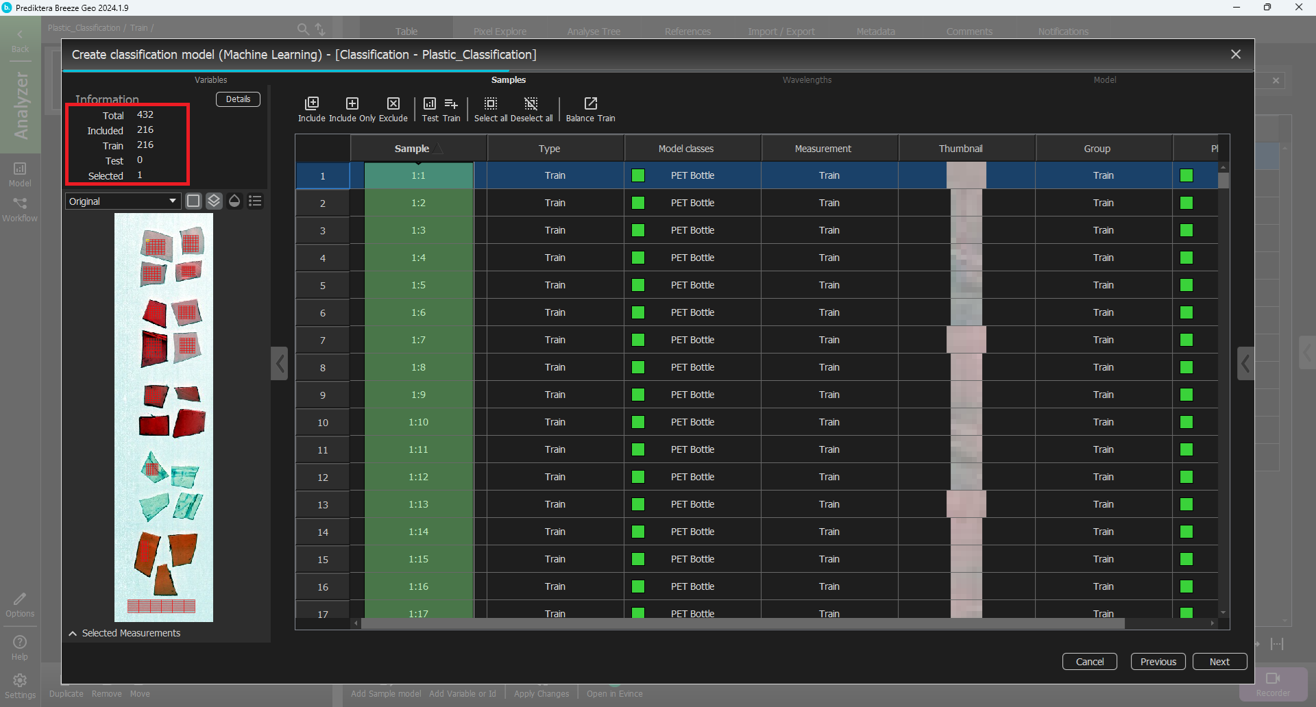
Click Select all and then Include.

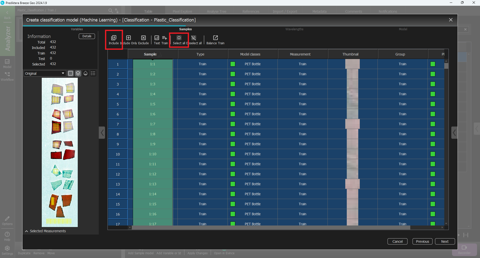
You can now see that the information changed and all the 432 grid parts are included in the train column.

Click Next.

In Step 3 press Next again.

In Step 4 of the modeling wizard you need to train the model again so click Train.

When the model is done click Finish.

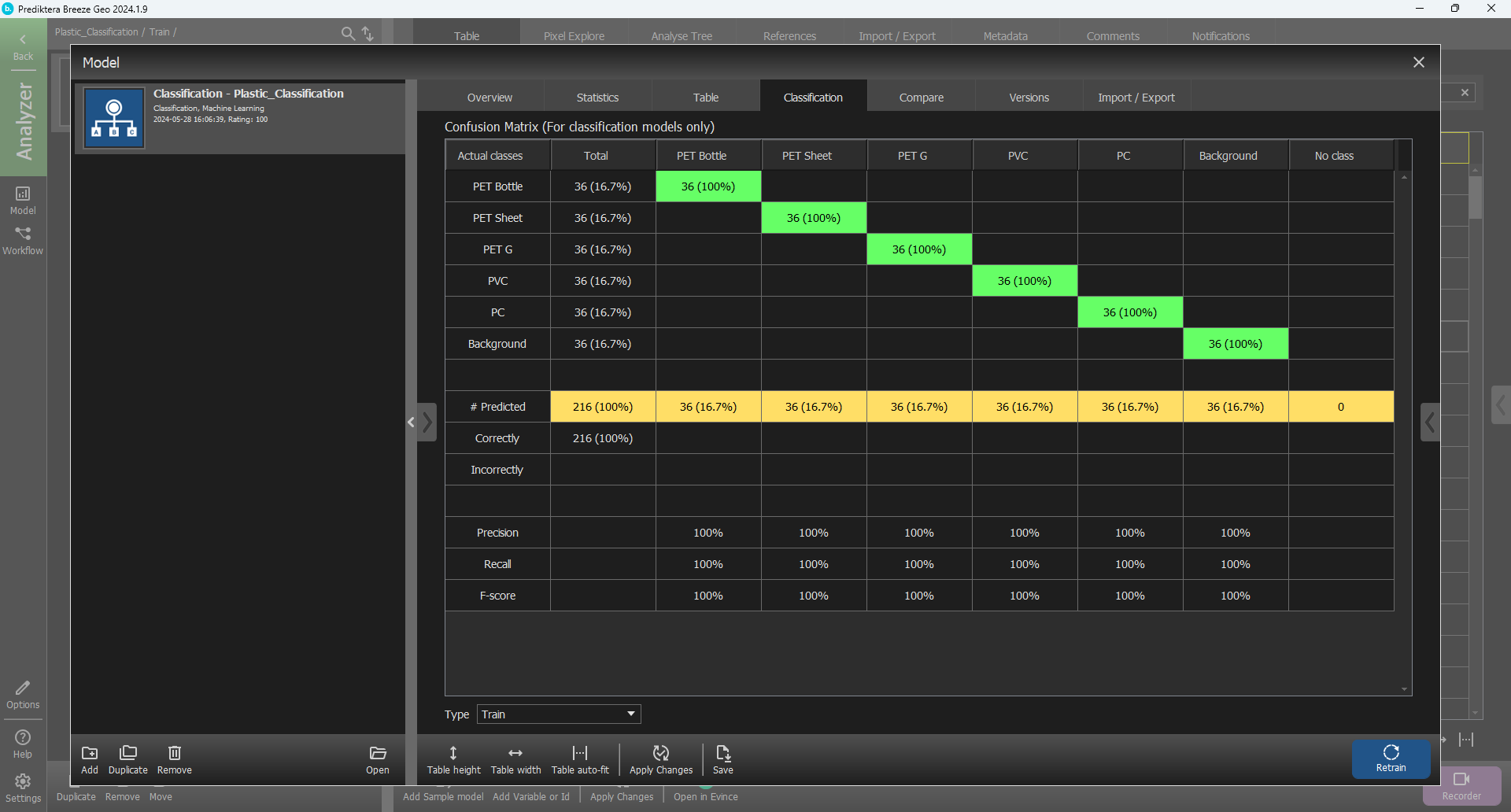
Close the model dialog and change the segmentation level in the table to Measurement, then select Apply changes.

Click the image corresponding to the classification.

You can now see that everything is correctly classified on the “Train” image. Let’s go to the “Test” image and see how the model is classifying those samples. Click Back to go to the Group level and select the “Test” image. Select Apply changes to see the classification. You should see results similar to the following image.

Simulate real-time prediction

Now that you have created a model, we need to prepare the simulated environment.

Click the Settings button.

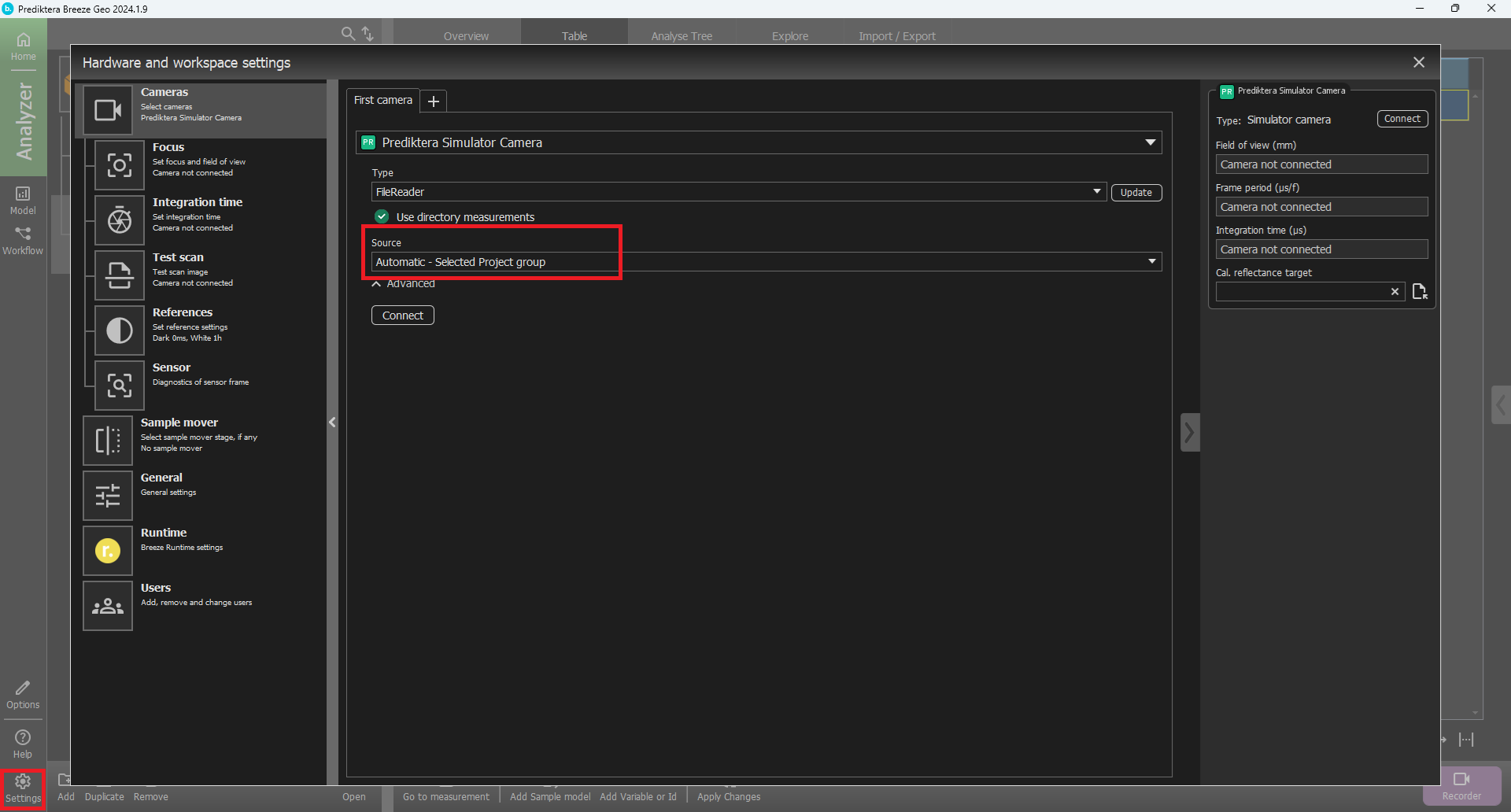
Select Cameras in the left table and make sure the Selected camera is Prediktera Simulator Camera, the type is FileReader, and the source is Automatic - Selected project group.

Then click Connect.

Once the camer is connected is connected, close the settings panel.

Open Workflow mode by clicking the button on the left sideo of the window, and select the Plastic classification project.

Click Add.

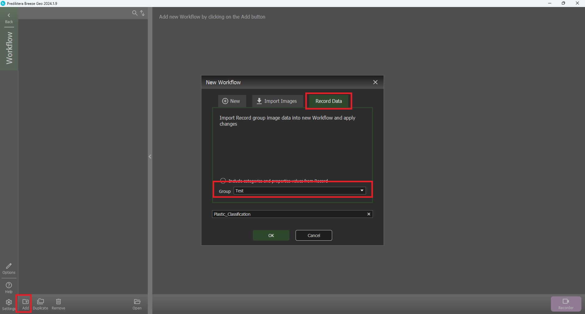
Select the Record Data tab and select the group “Test”. Click OK.

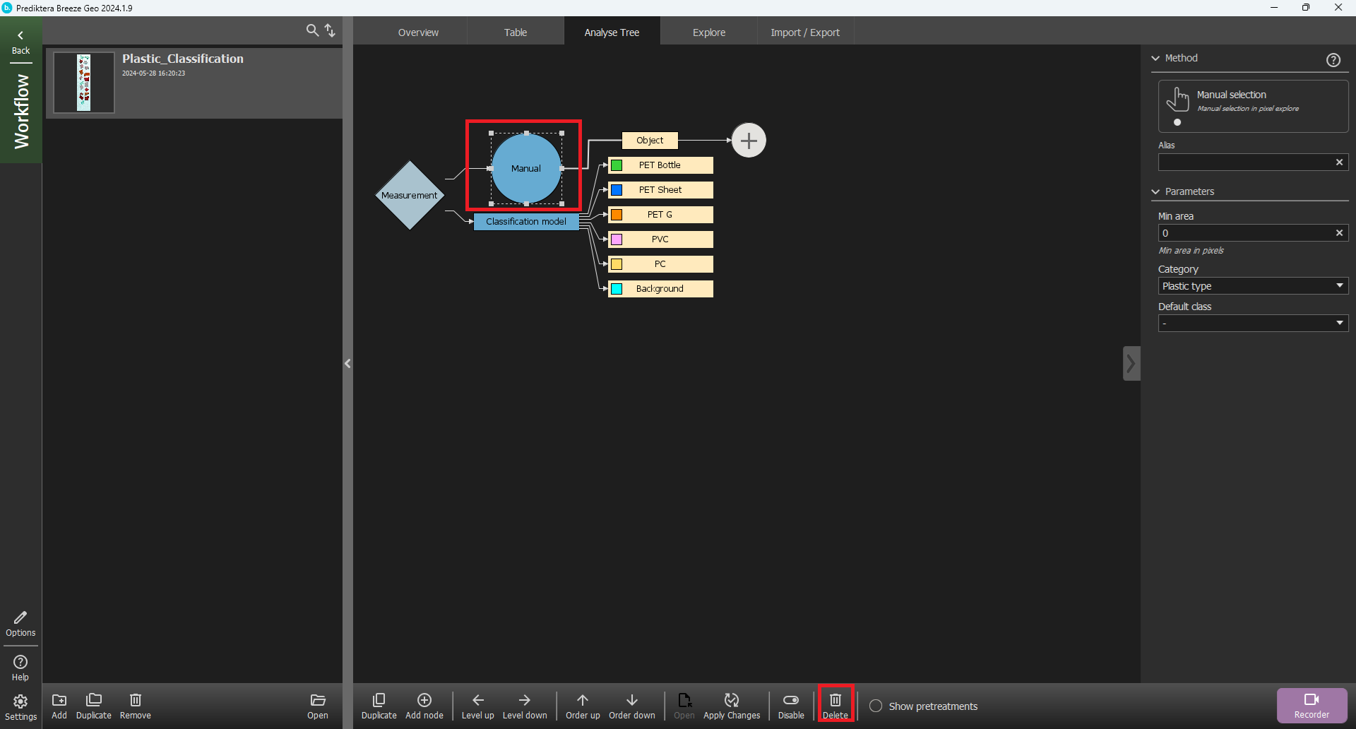
Go the the Analyse Tree tab and click on the Manual segmentation node and then click Delete.

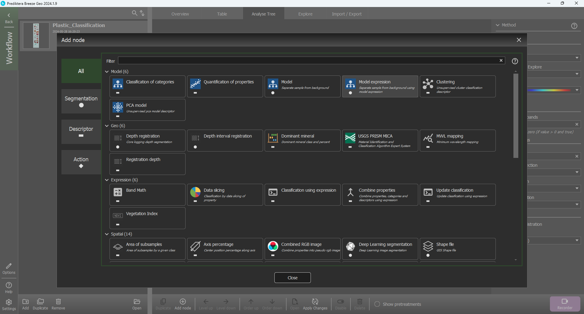
Click on the Measurement node, then the plus sign, then select Segmentation and choose Model Expression.

In the Expression field write Class != Background. This means that we will segment out pixels that are not from the Background class.

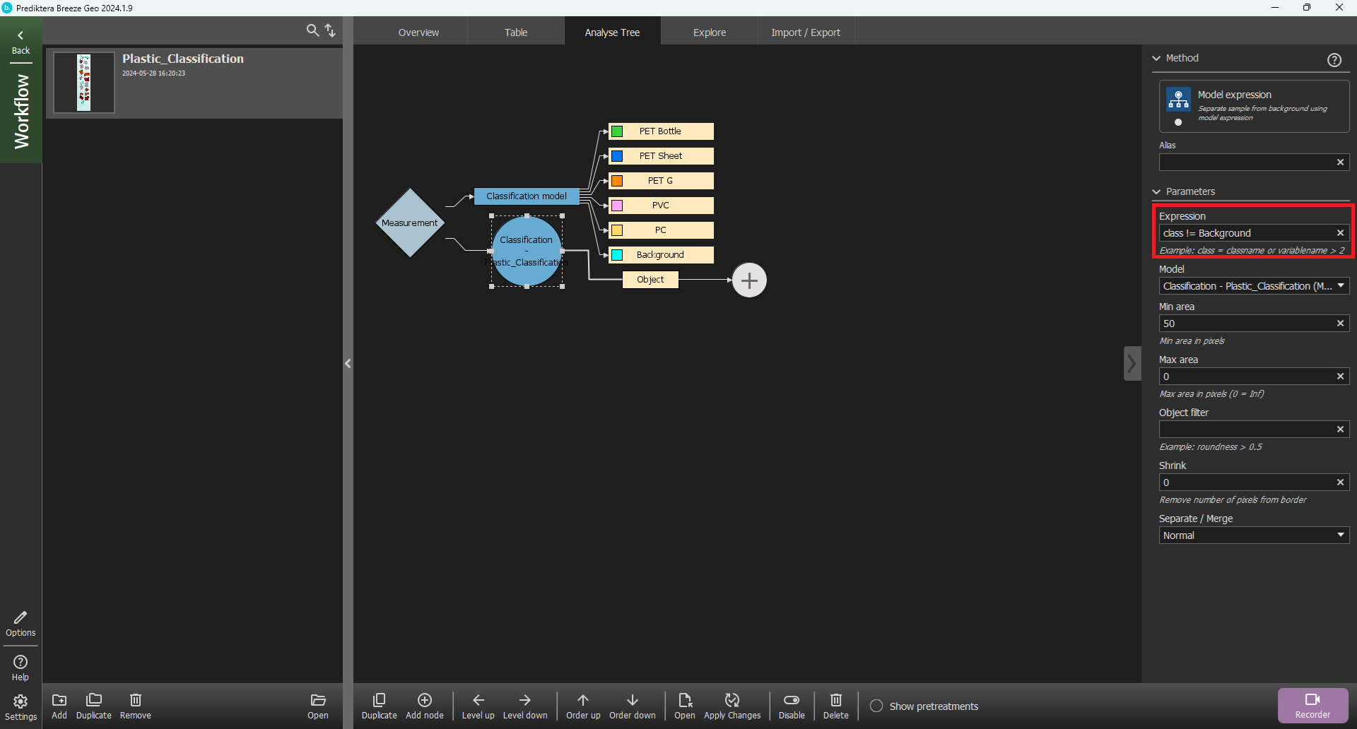
Click on the Classification model node and then click the Level down button to move the model to the end of the tree.

The model classification is now ready for real-time predictions. To test this, click on “Recorder” and the images from the “Train” and “Test” groups will be evaluated in a real-time scenario.

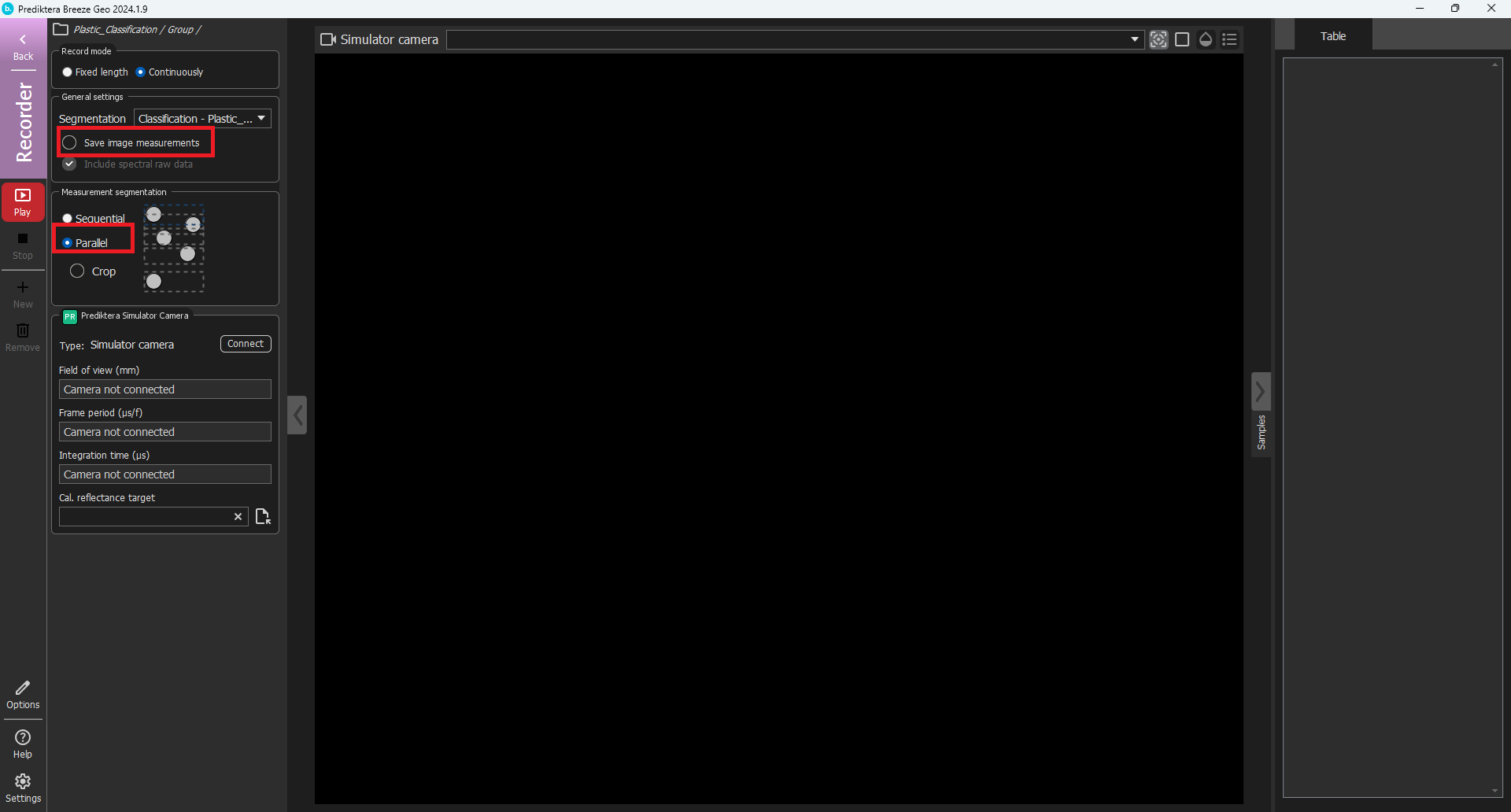
In Continuous recording mode, uncheck the Save image measurements option and select Parallel measurement segmentation.

Click Play.

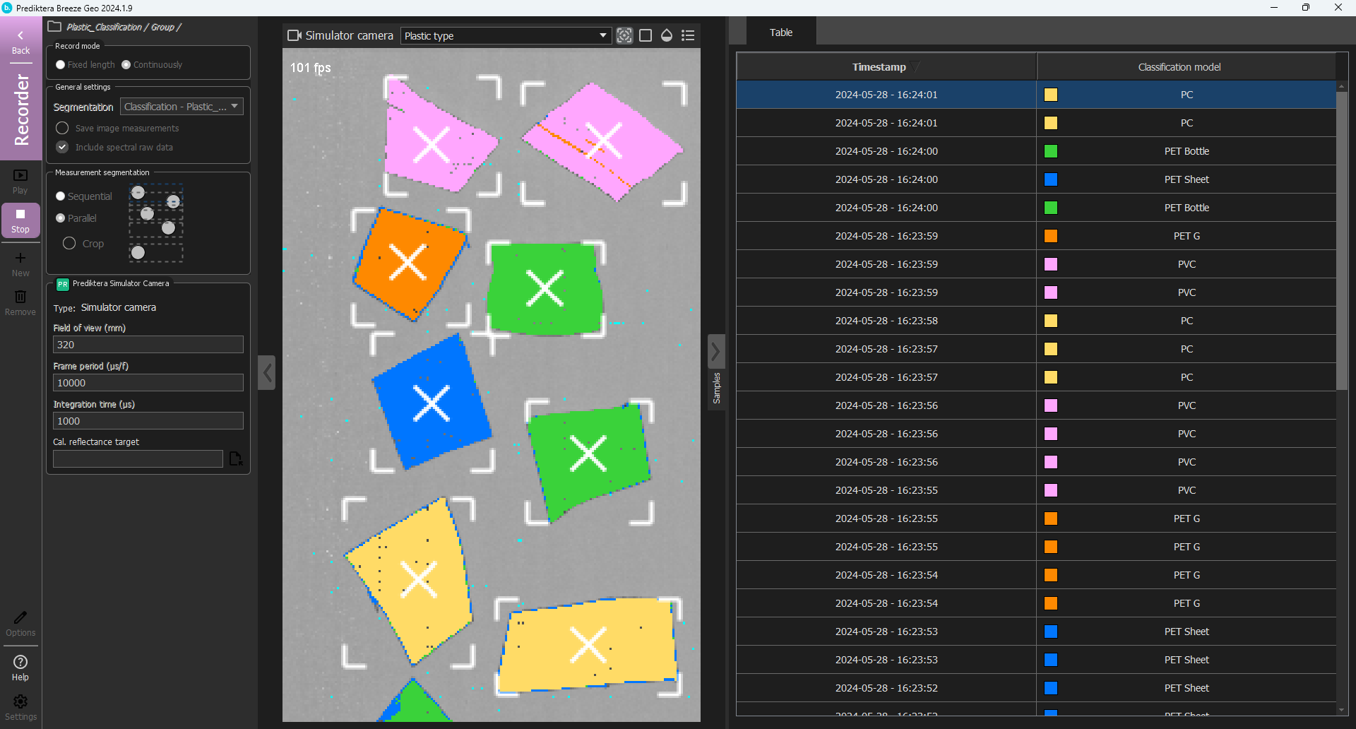
The data will now be analyzed in a real-time with automatic segmentation of the plastic objects.

Click the arrow button on the right side of the window to collapse the table of samples and give more space for the image.

You can turn on/off the settings for the blend, legend and target tracking for the visualization.

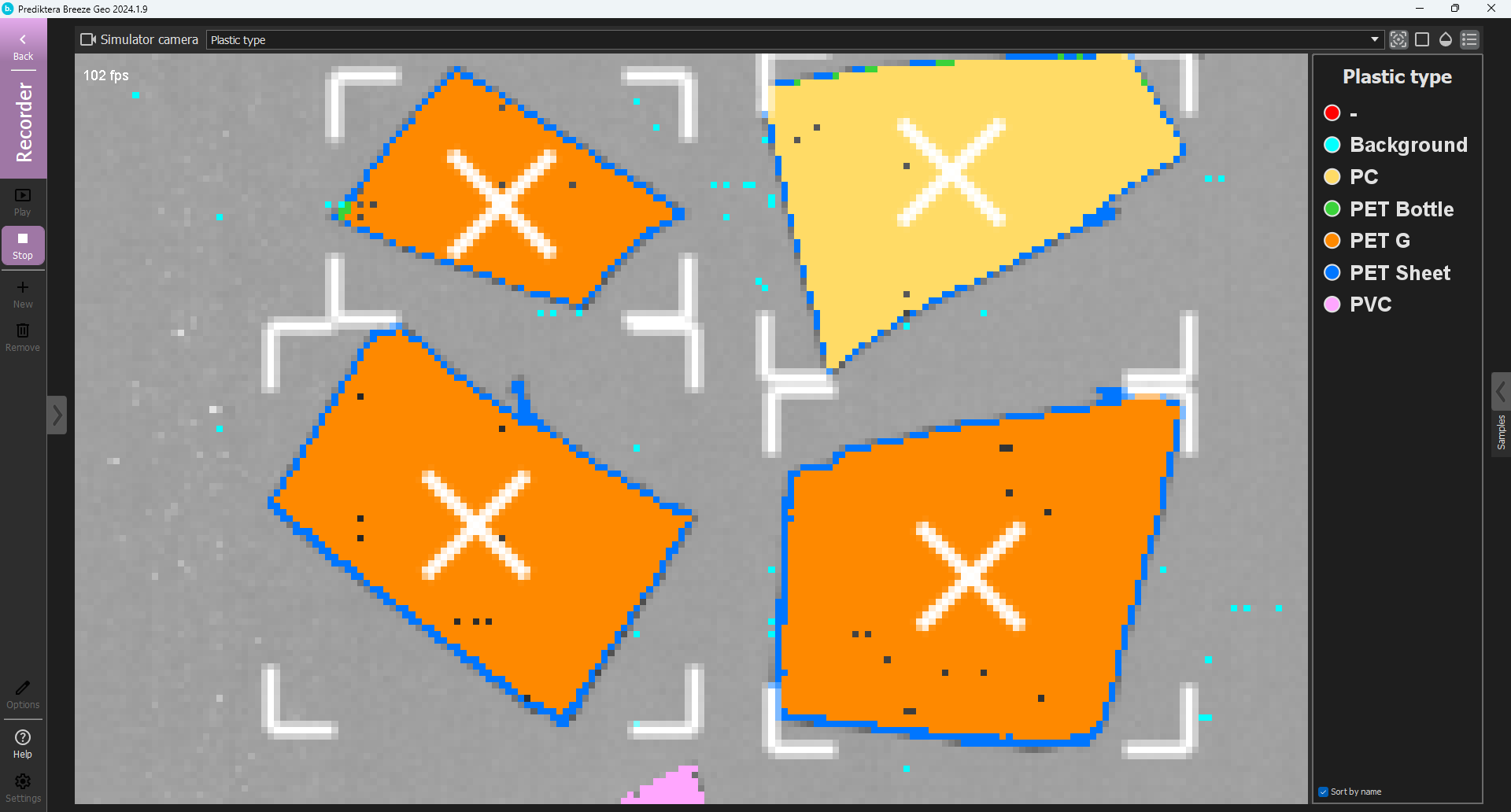
Good job! Watch the plastic classification roll by and receive a perfect classification. Click Stop to stop the predictions.