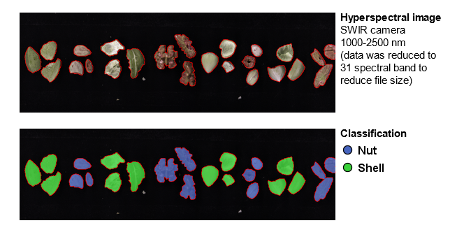
In this session, we'll use the same images as in the tutorial Intro to Breeze: Classification of nuts step 1 but add a new class variable to classify the type of nut. You will also test two classification model types (PLS-DA, SIMCA).
If this is new to you, we recommend you to go through step 1 first: Intro to Breeze: Classification of nuts step 1
Steps included in the tutorial
Import known class information to samples
Open up Analyzer tool.
For this tutorial, use the project Nuts_Classification.
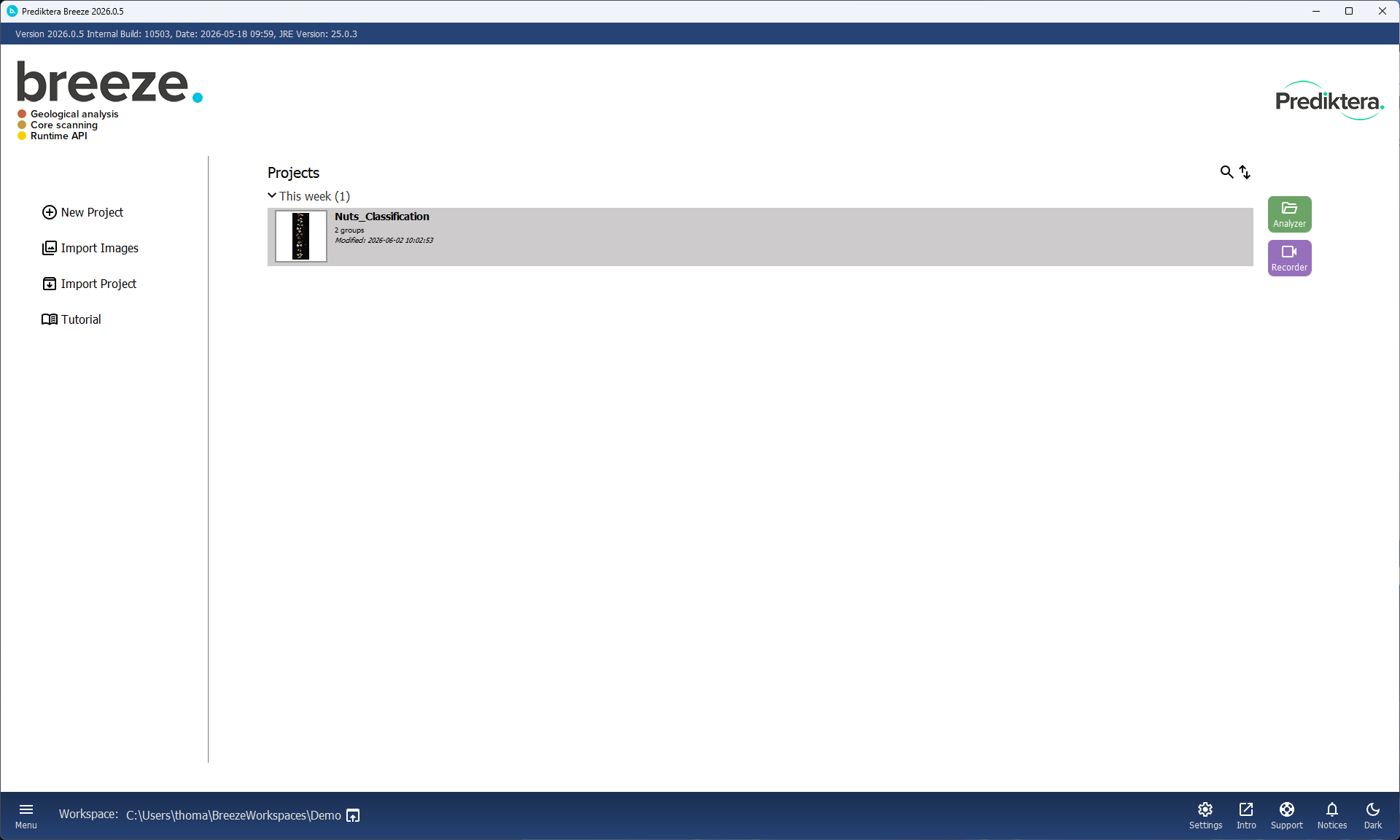
Select the project called Nuts_classification.
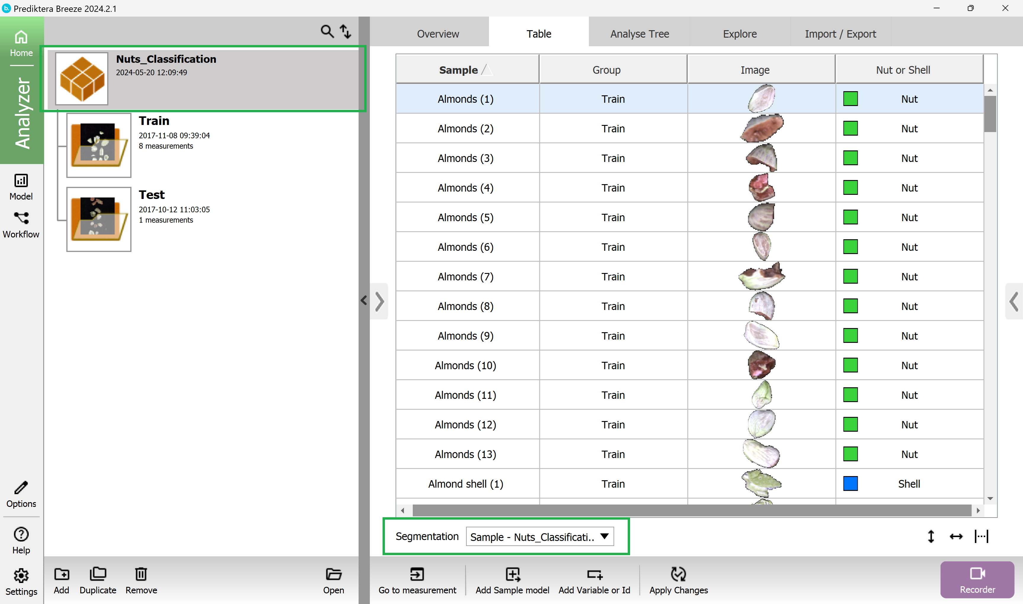
Select the Table tab.
Select Sample - Nuts_Classification in the Segmentation drop-down menu located under the table.
Import the “true values” to be able to model and predict data later.
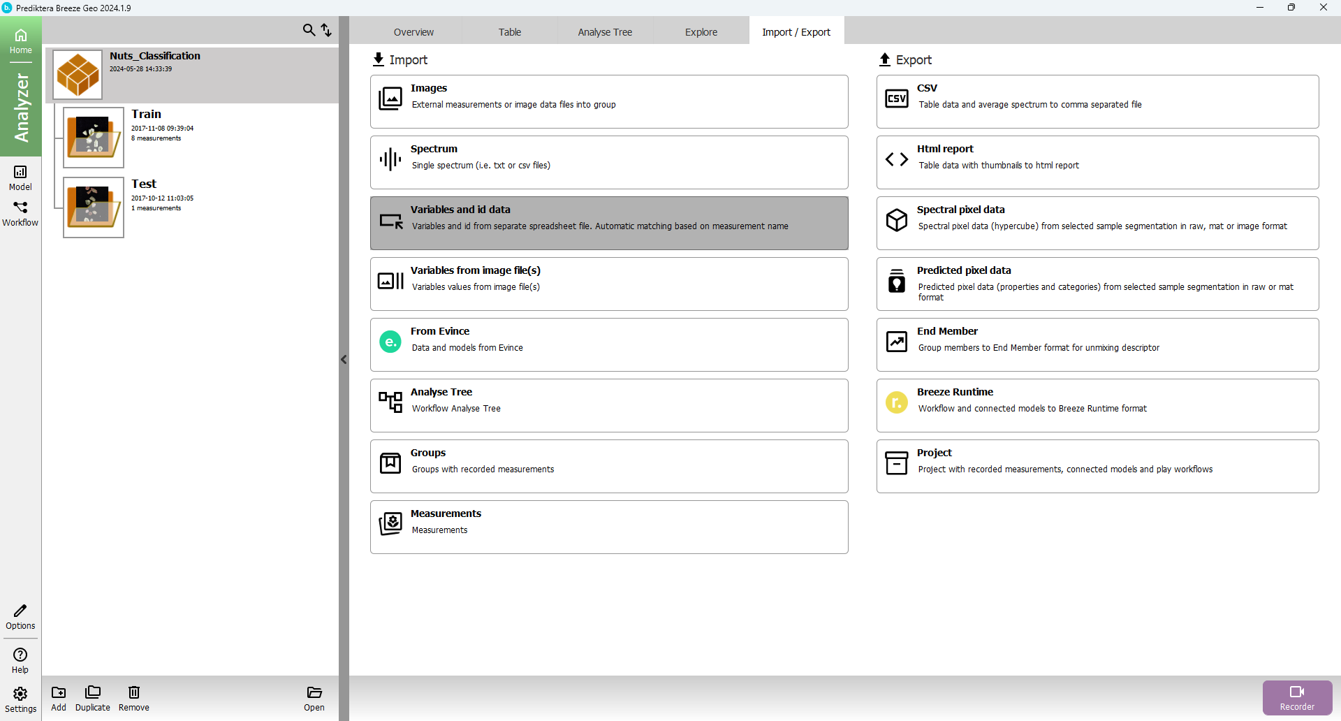
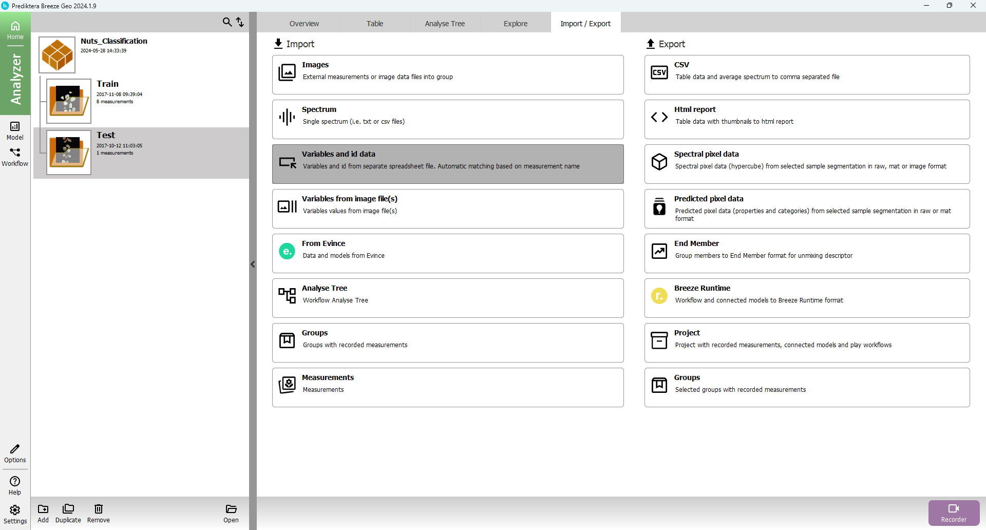
Select the Import/Export tab.
For this tutorial, we already classified the true values in the previous step. So now we need to fetch those files.
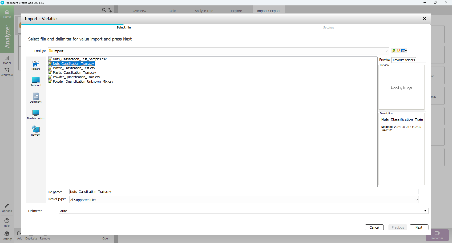
Select Import variables and id data.
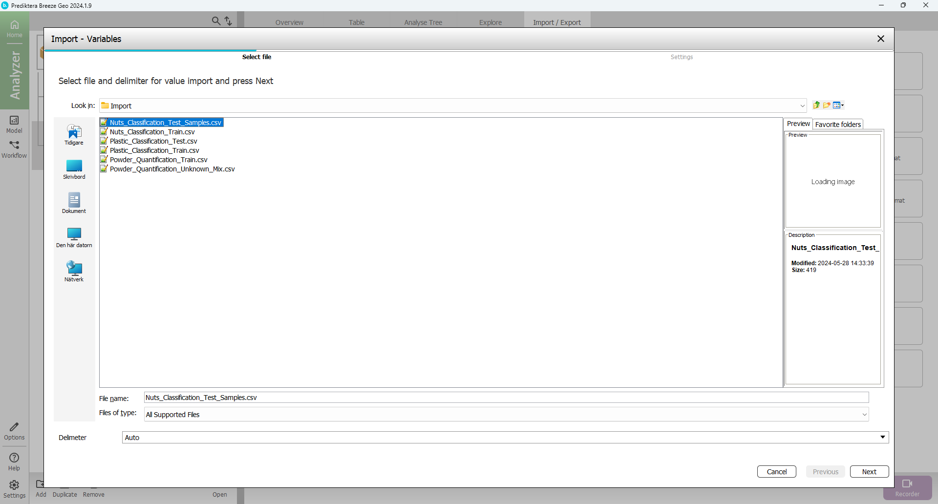
Choose “Nuts_Classification_Train.CSV”.
Select Next.
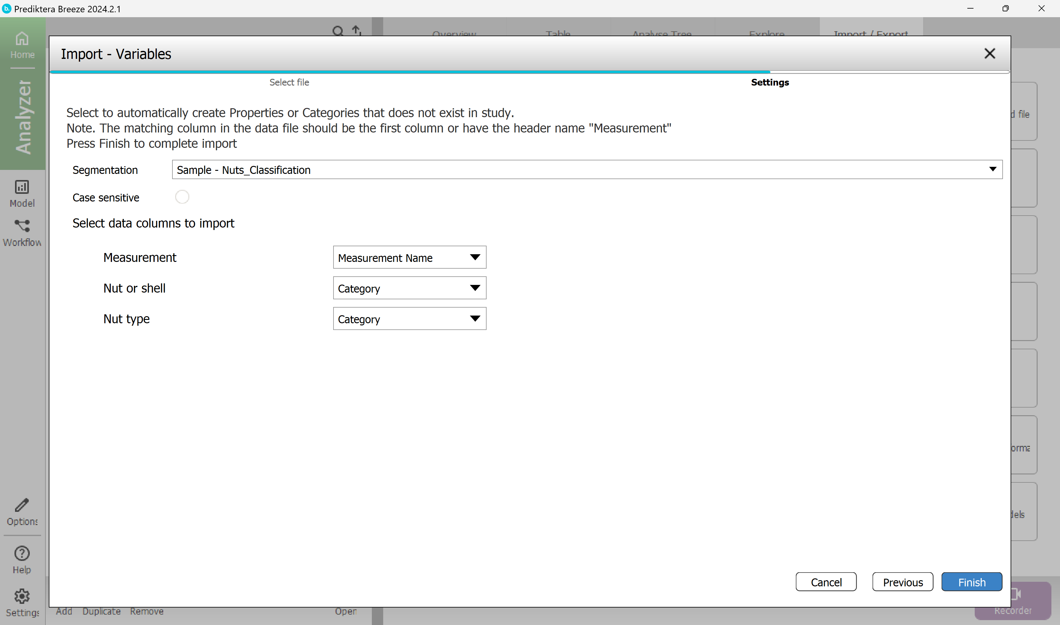
On the last page we can select the segmentation to import. For this tutorial, leave the last page unchanged.
Click Finish.
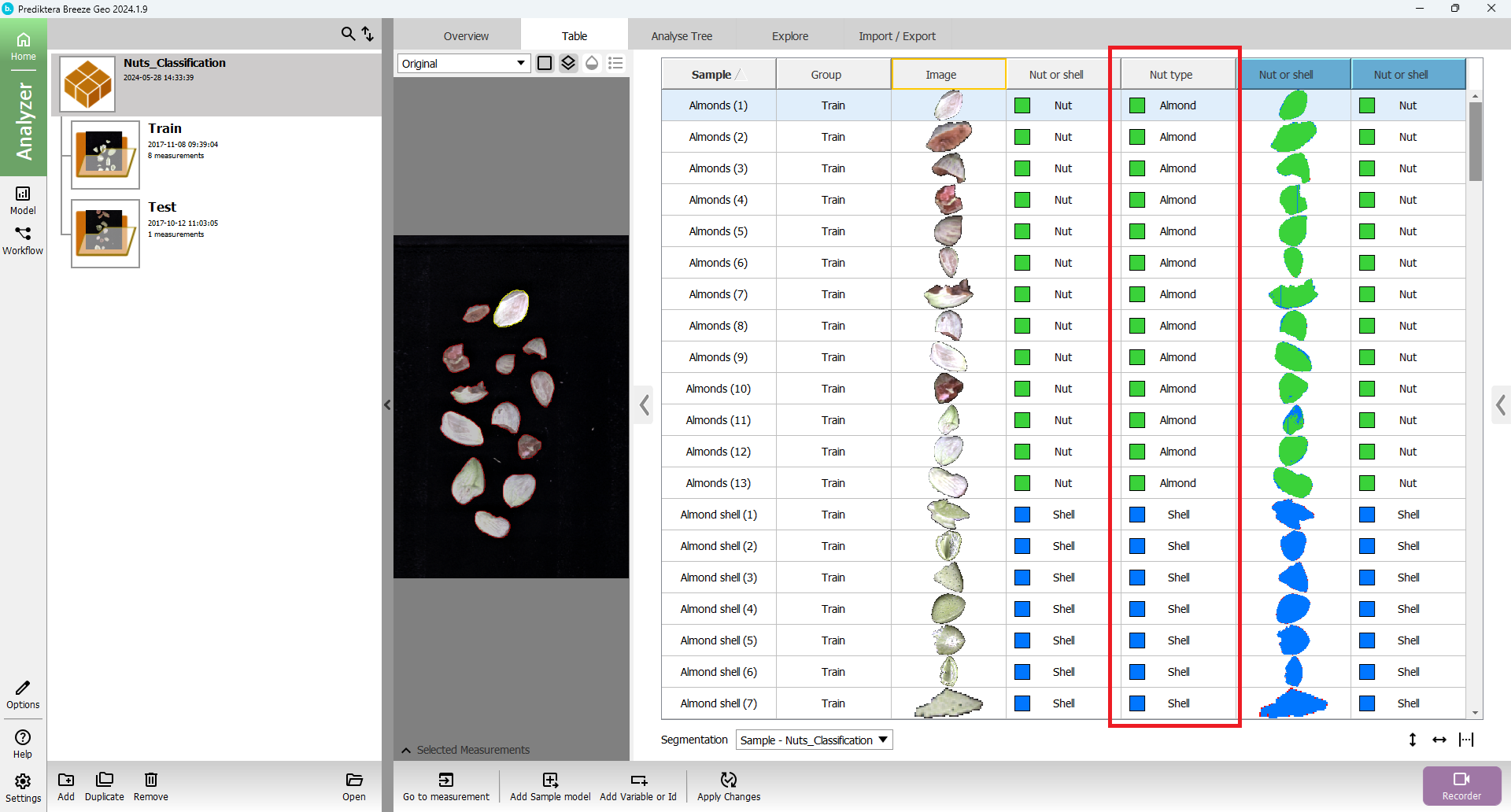
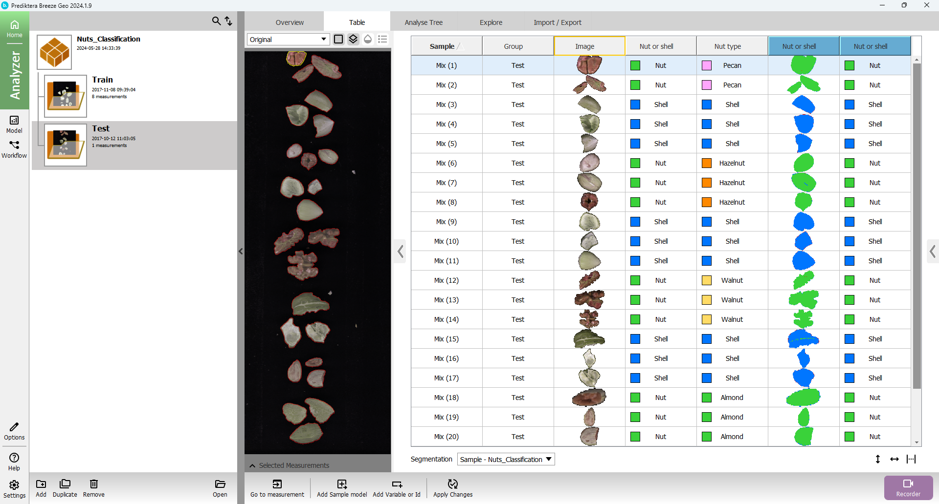
In the Table view, you should see the new Nut type class variable that was imported. The reference values were automatically matched with the correct sample object.
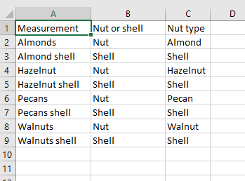
The spreadsheet .CSV file that you imported looks like this when opened in Excel. The column Measurement matches the class data (Nut or shell and Nut type) to the correct images and samples.
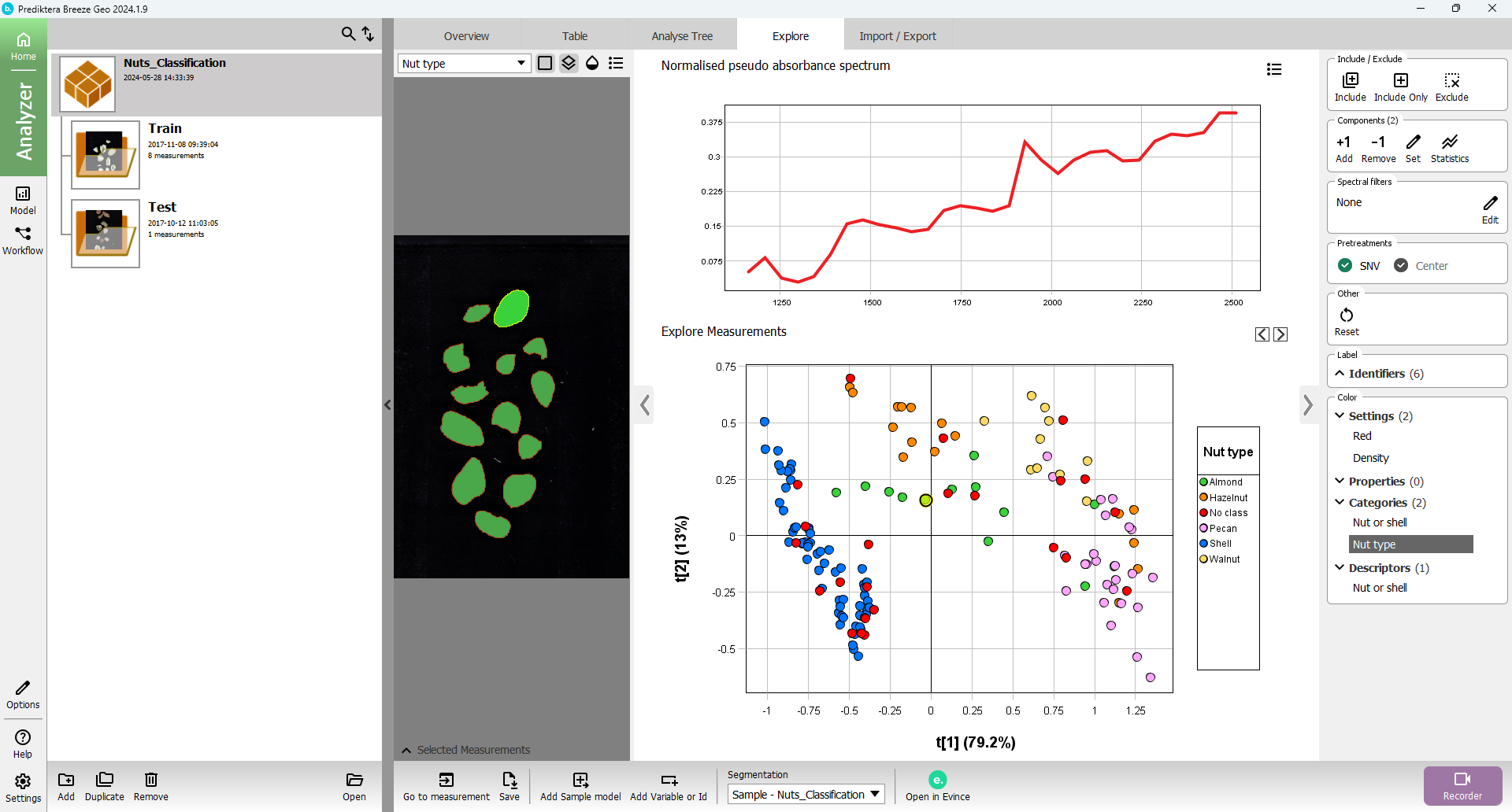
Open the Explore tab and then on the right side menu under Color, select Nut type to see how the different types cluster.
Create classification model (PLS-DA)
Now you will create a Classification model for “Nut type”.
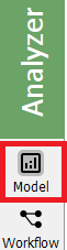
Open the model panel by clicking the Model button on the left side of the screen.
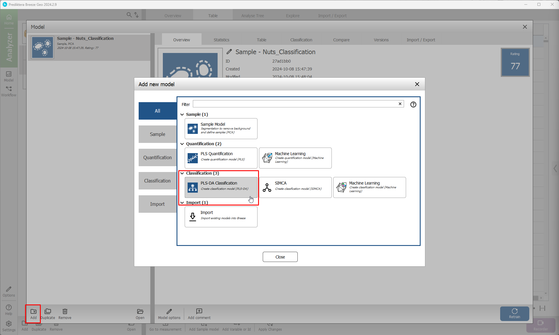
Select Add to make a new model.
Click on PLS-DA Classification.
Write a name or use the default one.
Select OK.
A wizard will be visible.
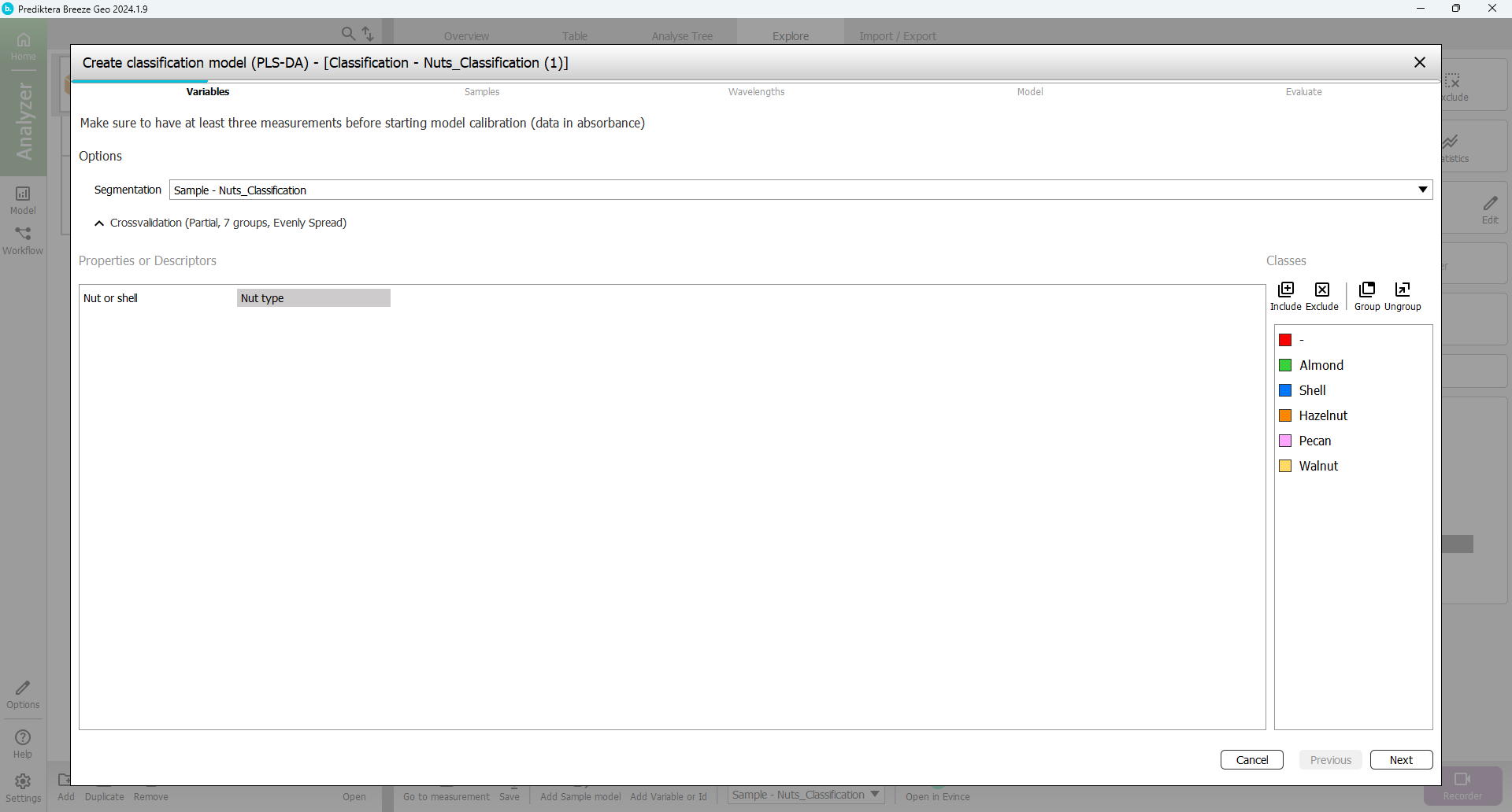
Step 1 - Variables
Choose the Nut type category.
Select Next.
For this tutorial: In the 2nd and 3rd steps of the model wizard just click Next (use the default settings) so that you come to the 4th step (Model).
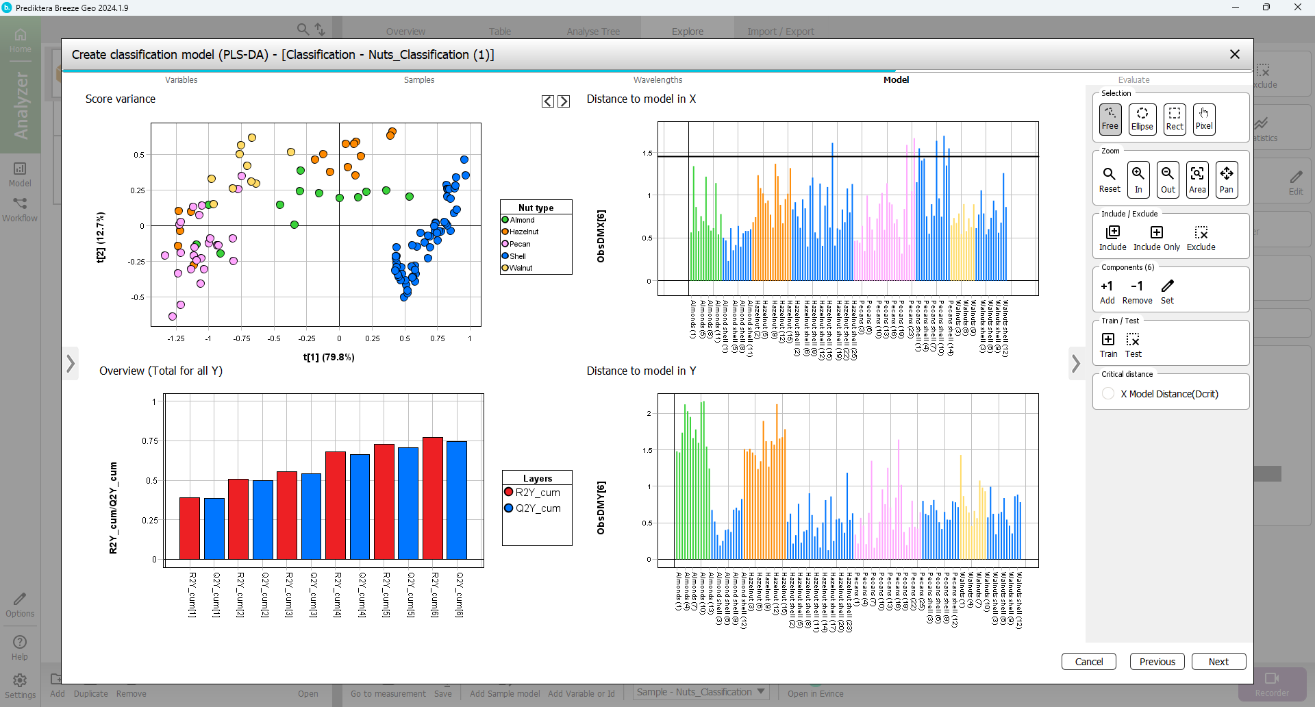
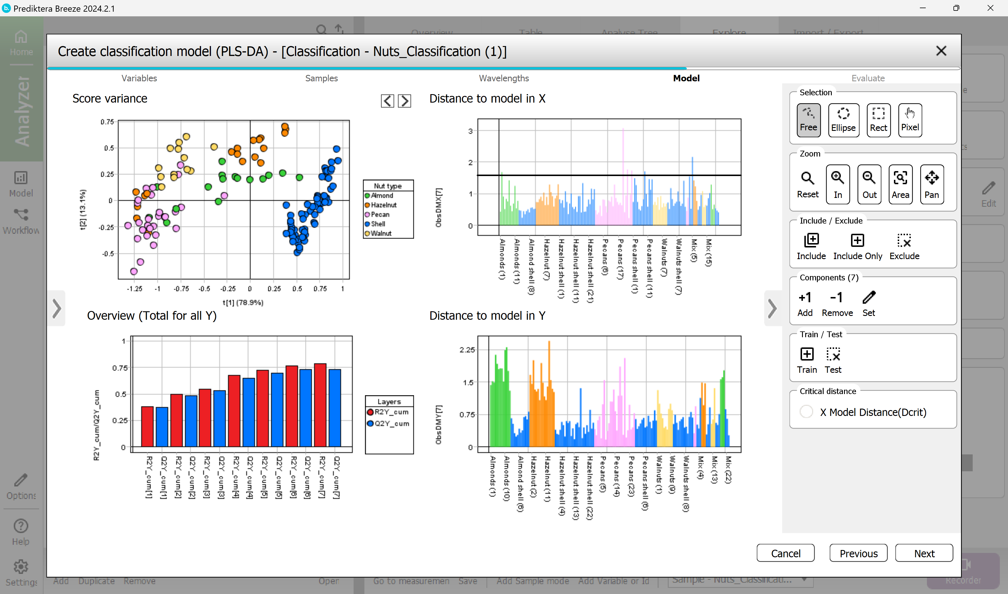
Step 4 - Model
In the Overview (total for all Y) you should have 6 components for your PLS-DA model.
Under Components you can Select Add to add more components to the PLS-DA model (to a total of 6, i.e. 6 red and 6 blue bars).
In Overview (total for all Y) you can see that the model has a R2=0.77 and Q2=0.73 by hovering the mouse over the bars.
Select Next.
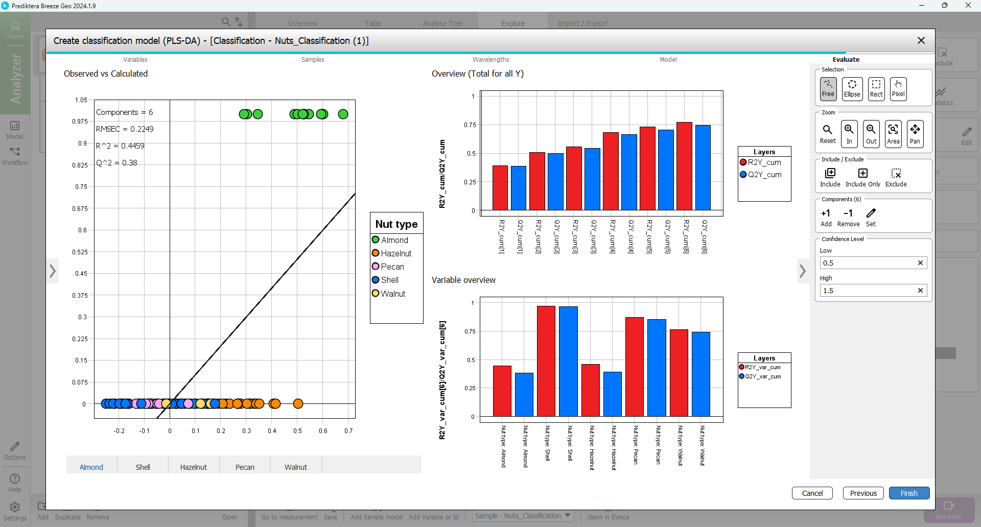
Step 5 - Evaluate
You can see the class separation by pressing the tabs for the different classes under the Observed vs Calculated plot. The Variable overview graph shows that Almond and Hazelnut could not be classified as well as the other types.
Select Finish.
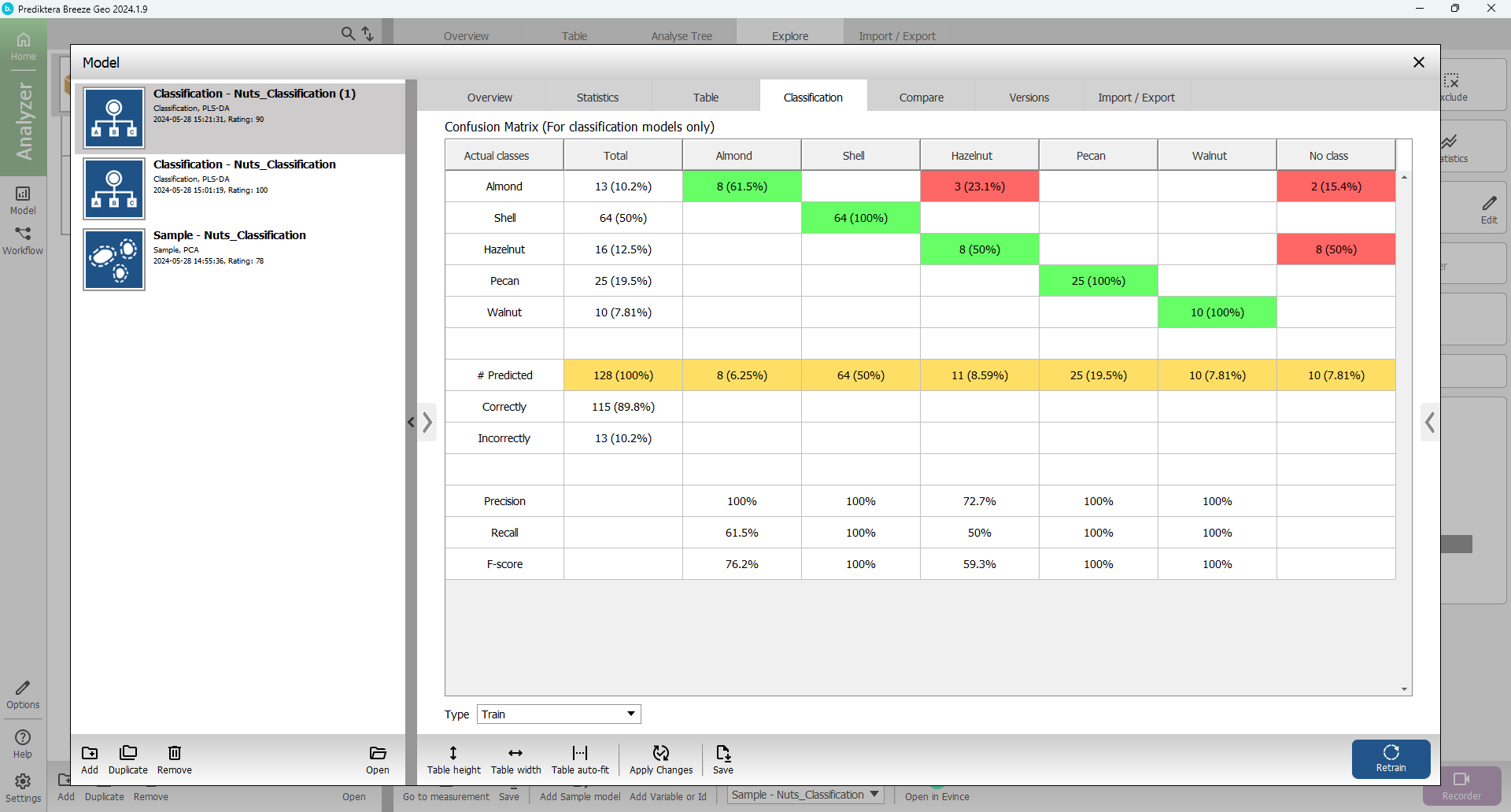
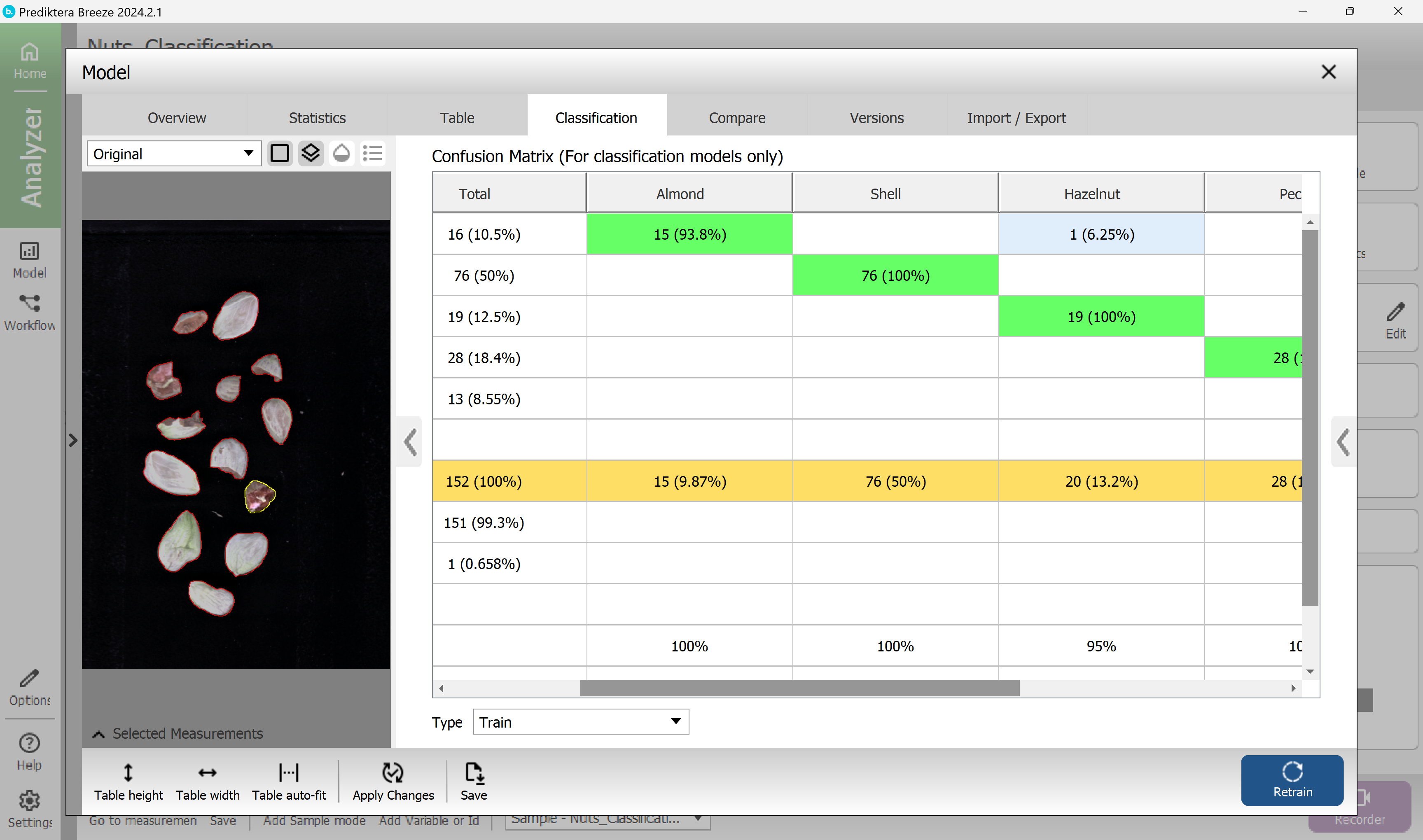
Select the Classification tab to see how well the training data was classified by the PLS-DA model (the results might vary slightly depending on how you did your sample model).
In this example, 3 of the Almond samples are misclassified as a Hazelnut and 3 as No class. For the Hazelnut there are 8 samples that are incorrectly classified as No class.
Create classification model (SIMCA)
Let’s compare the PLS-DA model with a different classification model type.
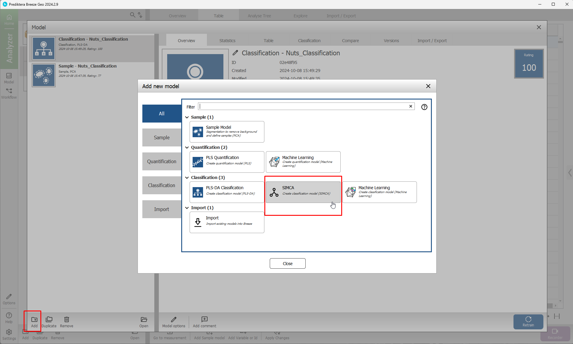
Select Add
Select SIMCA
Choose a name for the model or use the default one.
Select OK.
Choose Nut type

In the 2nd and 3rd steps just click Next (use the default settings).
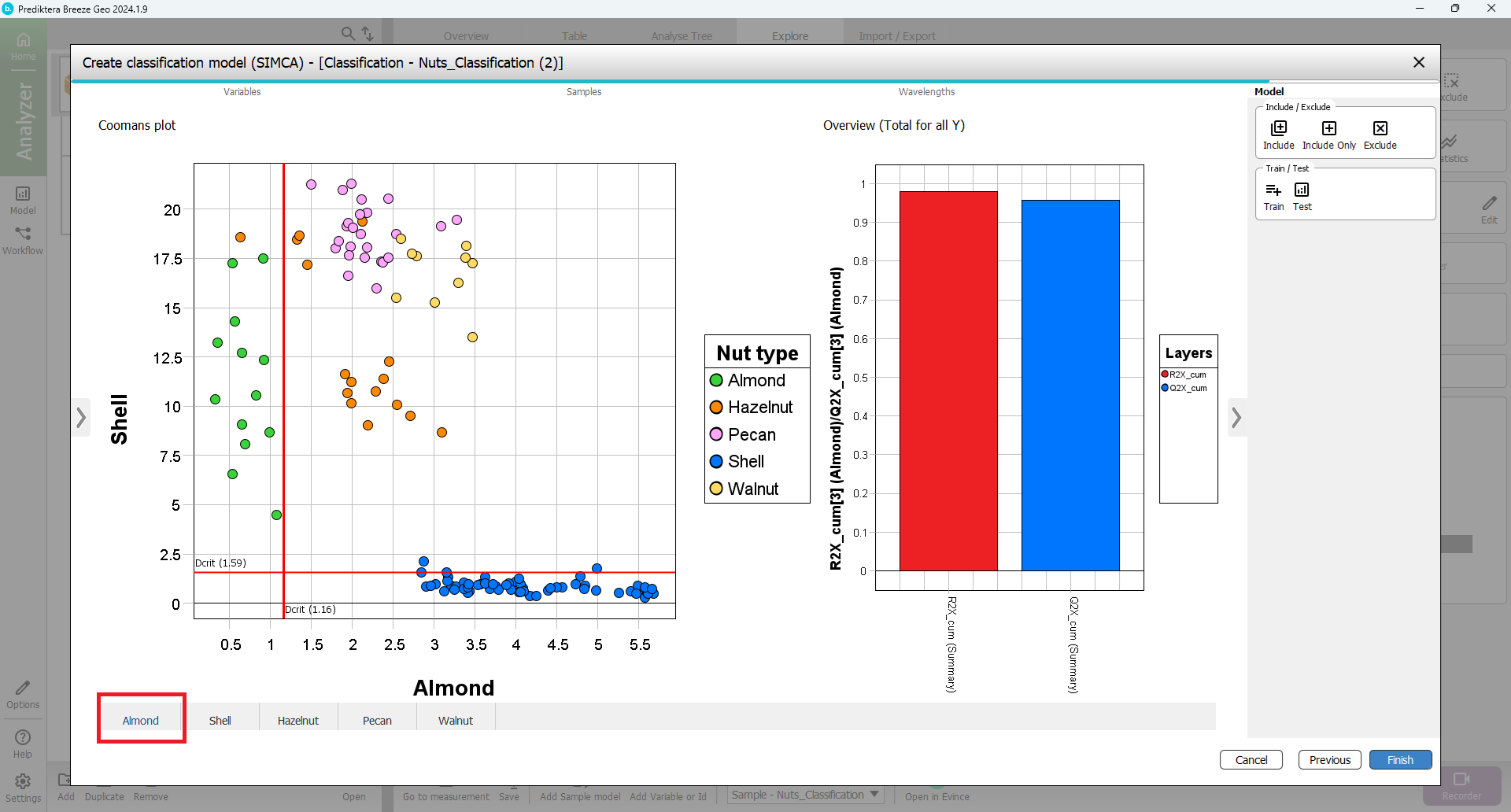
In the SIMCA method, one PCA model is created for each class.
All samples are then compared to that class model to determine if they belong to that class. In the Coomans plot, you can set the critical distance for each class model. If a sample is inside the critical distance it belongs to the class.
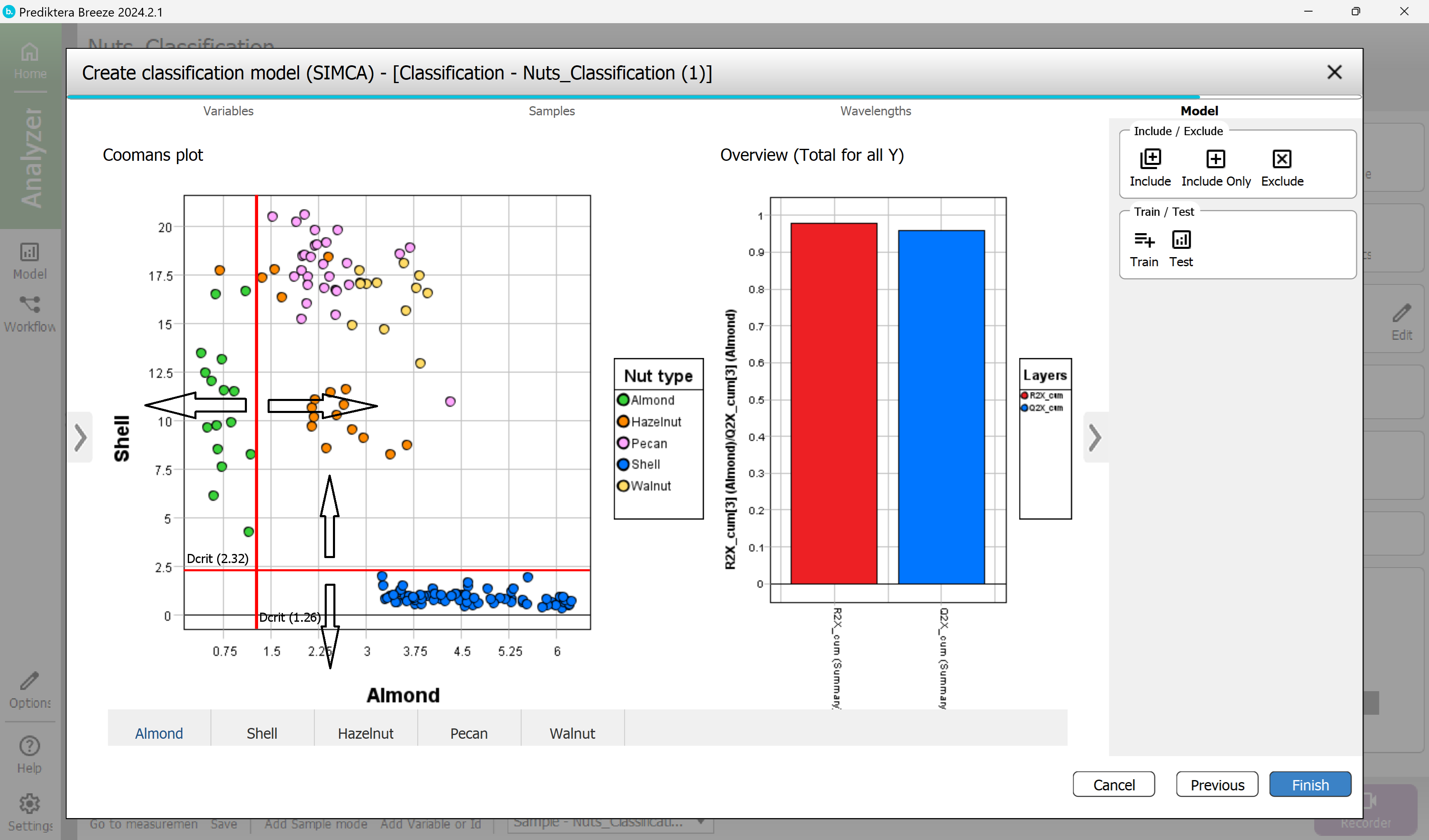
a) Select the class model for Almond by using the tabs under the Coomans plot
b) Drag the vertical red line to adjust the limit to include all Almond samples (but as few as possible of the other samples). Samples to the left of the red line are included in the Almond model.
Press the tab for each of the classes and repeat the steps in a) and b)
Overview (Total for all Y) is only showing how well each class model can explain the samples in that class. It does not show how well it can classify other samples)
Select Finish to complete the model
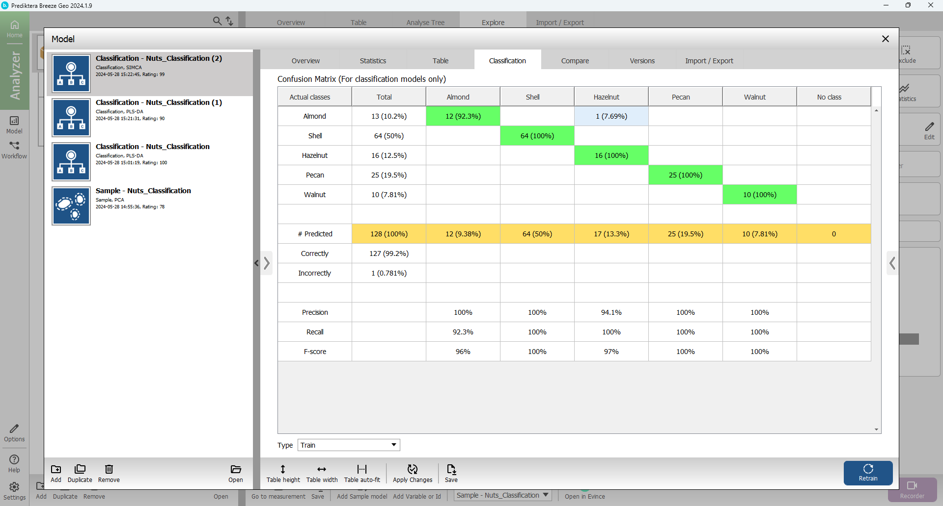
Select the Classification tab to see how well the samples in the training data were classified.
Press the arrow to maximize the table view and the arrow to open the preview image.
Click on a field in the table to see the corresponding samples in the preview image.
In this example, with the SIMCA classification a total of only 1 samples were misclassified (you might get slightly different results depending on how you set the critical distance in the previous step). This can be compared to 14 misclassified samples for the PLS-DA.
Import the known class information for the test samples
To validate the model you should use an external test set to see how well it can classify samples that were not in the training data set. We will now add the known class information to the image Mix in the Test group.
Close the Model window
Open the Nuts_Classification project.
Select the Test group
Select the Import tab
Select Variables and id data
Select Nuts_Classification_Test_Samples.csv.
Select Next.
Use the default segmentation and click Finish.
The table should look like this for the Test group.
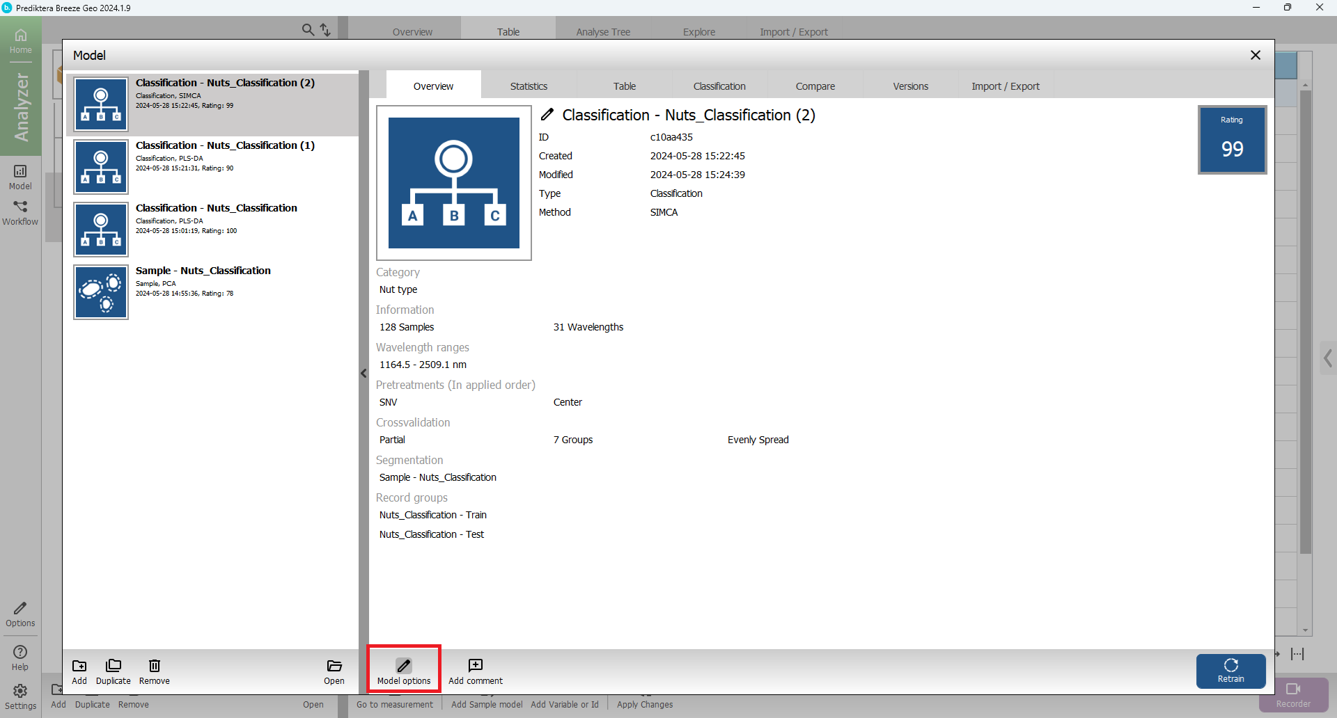
Click the Model button
and with the SIMCA model selected
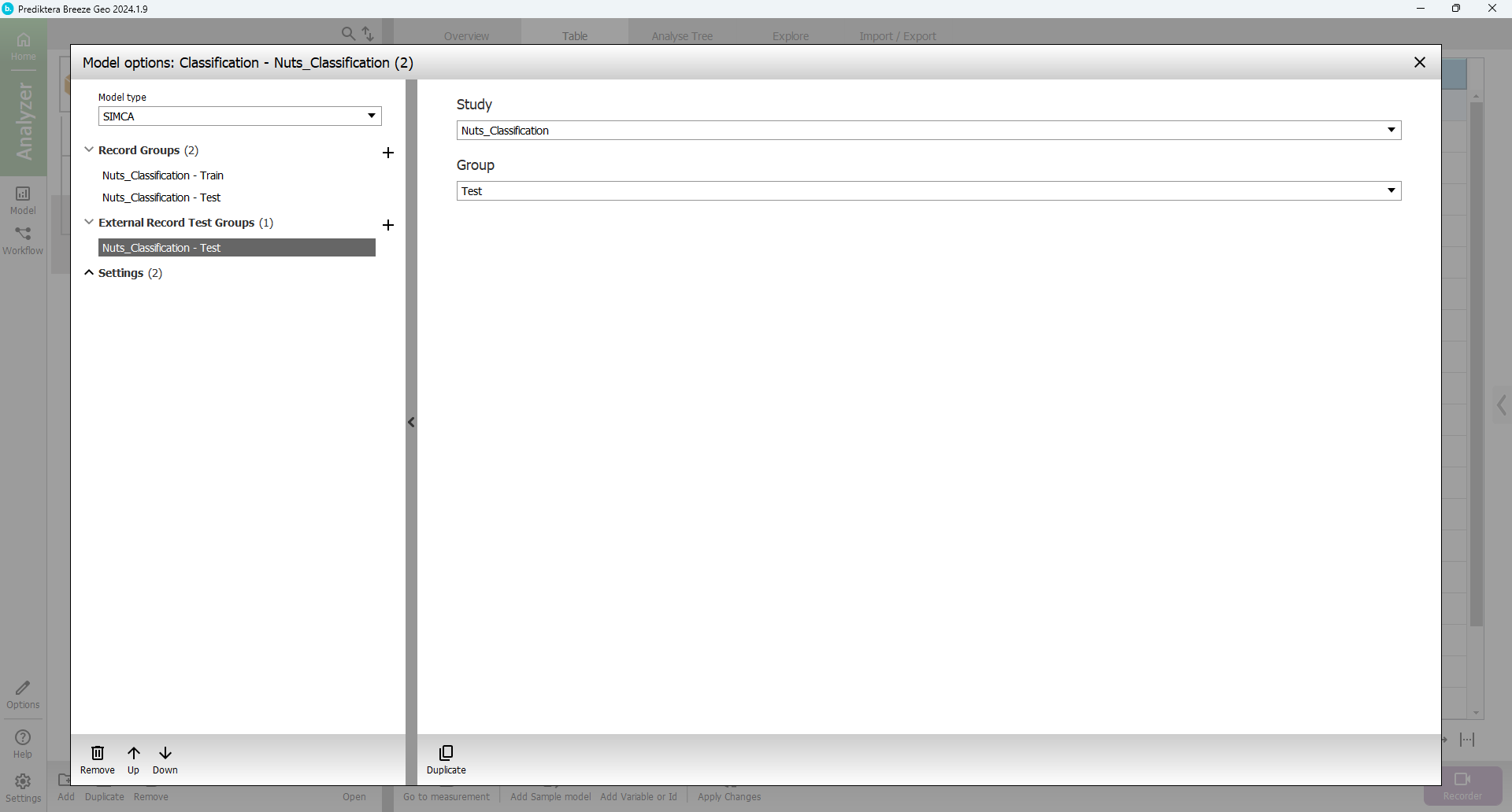
Press Model options
Click the plus sign to Add External Record Test Group.
Make sure the group named Test is selected in the menu on the right.
Close the dialog
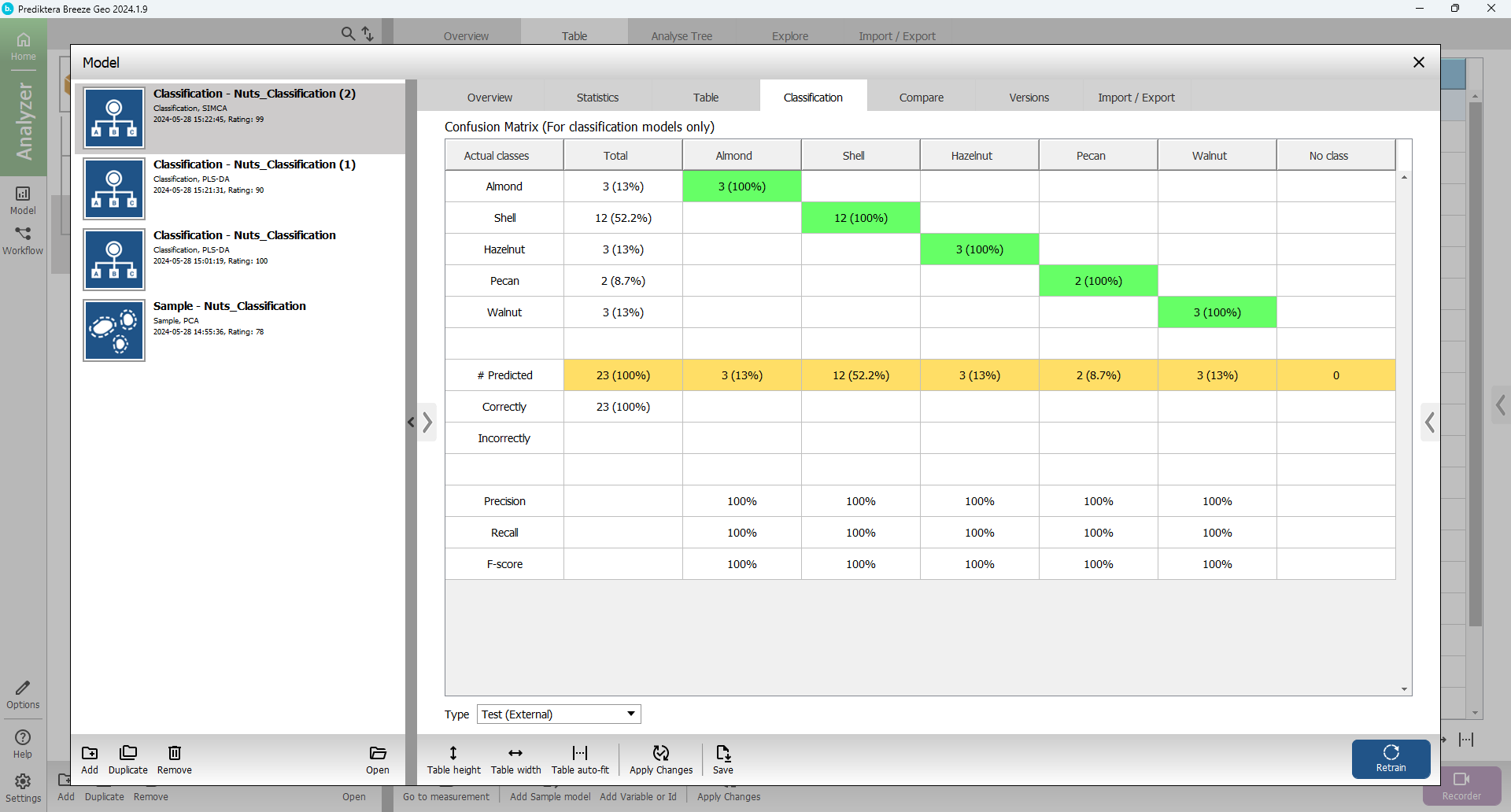
Select the Classification tab
Select Test (External) in the drop-down menu under the table.
You can now see how well the SIMCA model could classify the 23 samples in the Test group.
Let’s see how well the PLS-DA model can classify the test set.
Select the Classification - Nuts_Classification(1) PLS-DA model.
Go to the Overview tab.
Click the plus sign to Add External Record Test Group.
Make sure the group named Test is selected in the menu on the right. (just like you did for the SIMCA model)
Open the Classification tab
Select Test (External) in the drop-down menu under the table.

Create workflow and Import Record test data
Now let’s test the new models for Nut type in the Workflow mode.
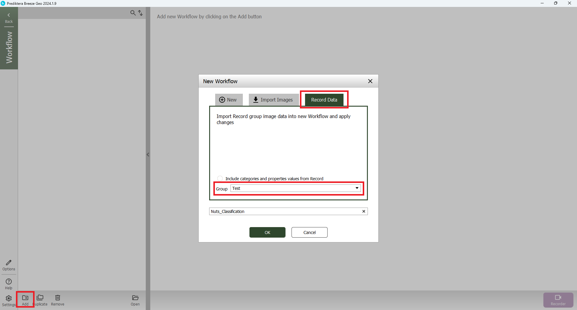
Open up Workflow.
Select the Add button.
Select the Record data tab.
Select Test from the drop down called Group.
Select OK.
By default Breeze applies the latest model that you have in Model in the workflow.
In this case the SIMCA model.
Open Analyse Tree tab.
In the Analysis Tree, you can see the steps in the workflow from left to right.
First, the Measurement is analyzed by the Sample model that finds the samples (Object).
Each Object is then analyzed by our model and then classified into different classes.

Click on the blue symbol for the Nut type model (the model that classifies into the Nut or shell classes)
Click Duplicate button below in the tool bar.
The Nut Type model has now been copied and added to the Analyse Tree.
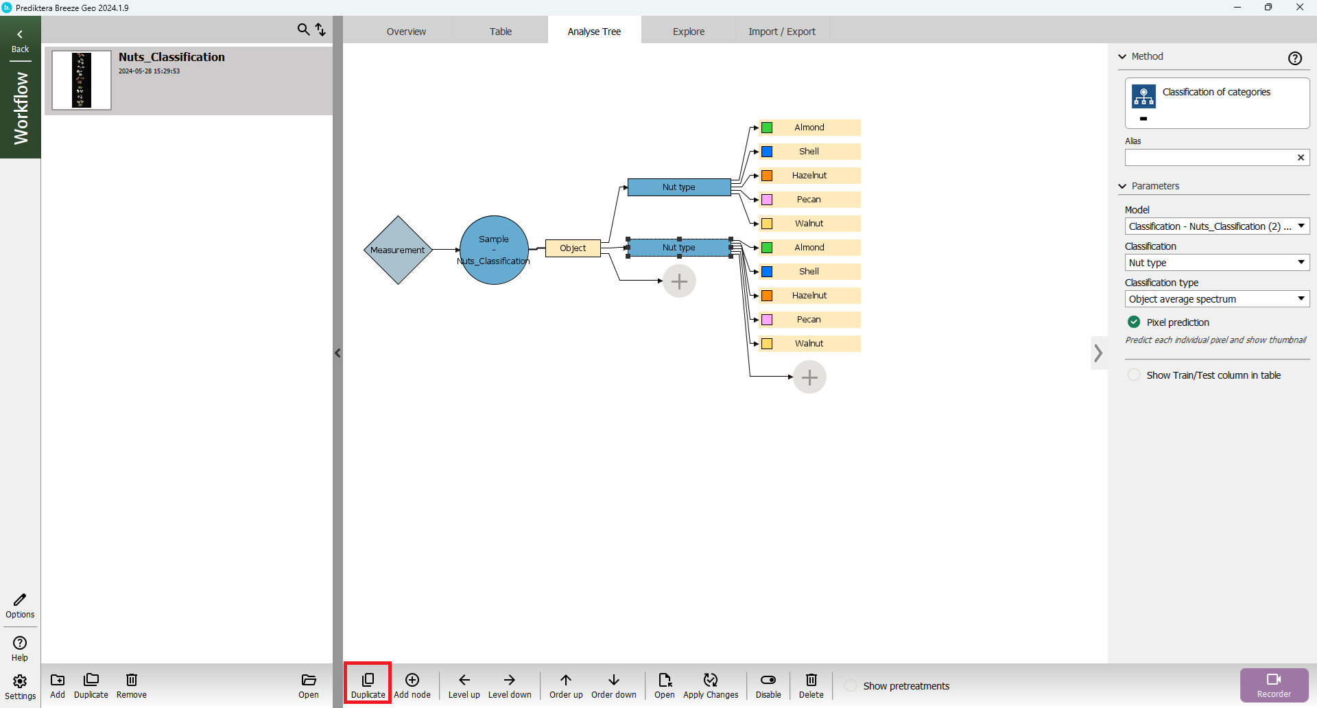
Click on the first Nut type model to see the settings menu for that model on the right side (drag the vertical line to adjust the size). In this menu, you can see the settings for the selected Node in your Analyse Tree.
In the Model drop-down select the SIMCA model. In the Alias field, write “SIMCA” and press enter on your keyboard.
Click on the 2nd Nut type model in the Analyse Tree and change it to use the PLS-DA model in the Model drop-down menu. Write the Alias as “PLS-DA” and press enter. As you can see the text for each model has now been updated in the Analyse Tree.

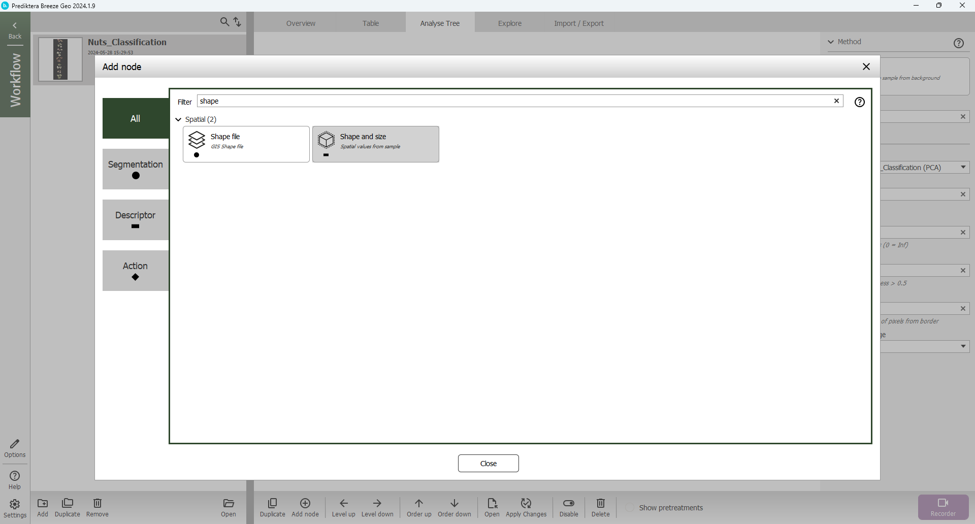
In Breeze, you can add many different types of descriptors to your workflow. Click on the sample model in the Analyse Tree and then select the plus sign.
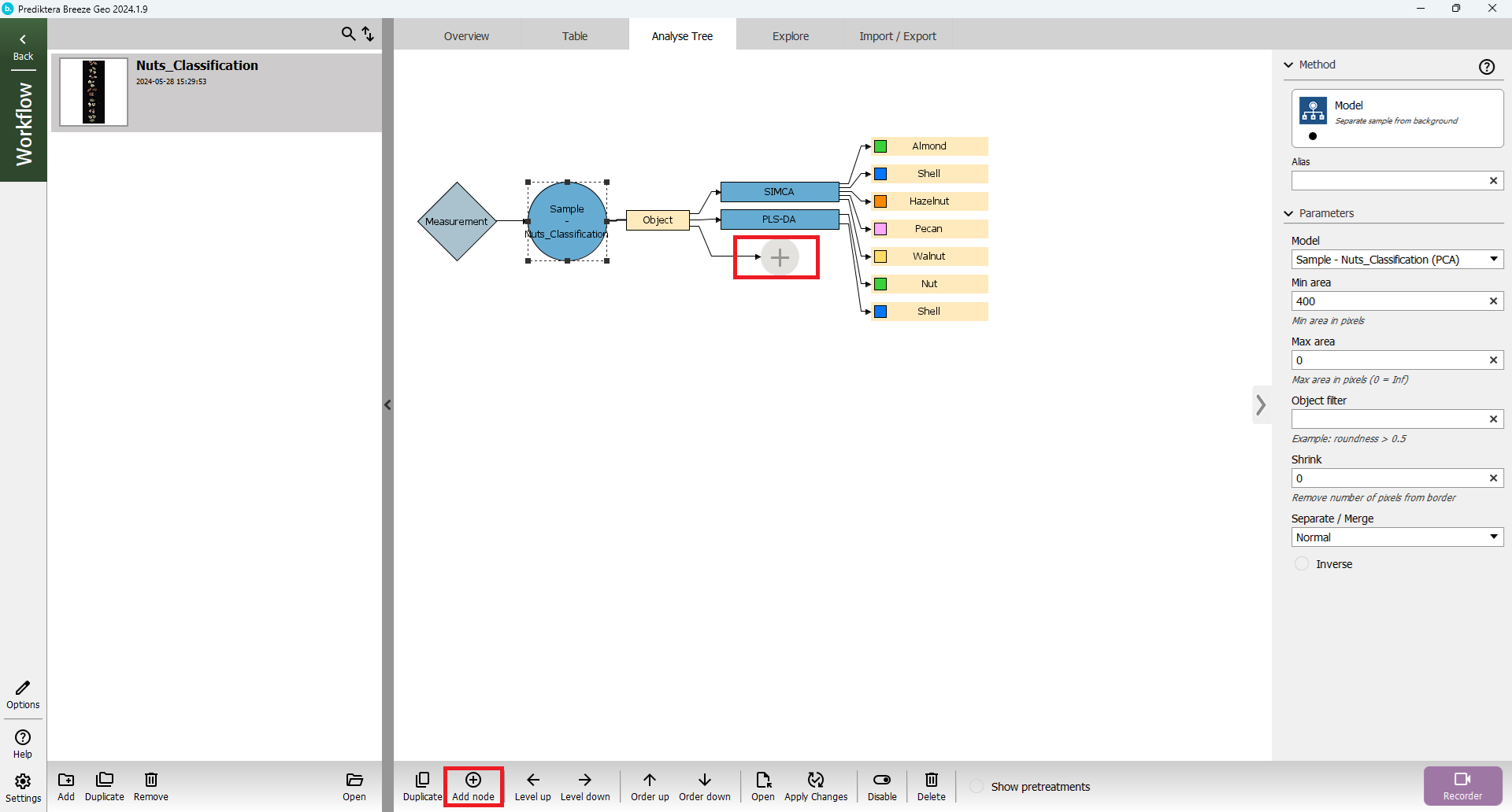
A new Node has now been created as a subnode under the Object generated from the Sample model. In the Add node menu you can see the different types of descriptors that are available in Breeze. Select Shape and size(you can search for descriptors using the Filter field).
The default Output is Area.
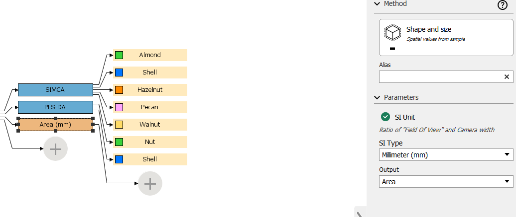
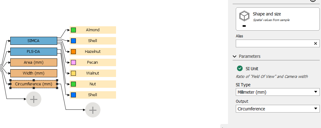
With the Area node selected in the Analyse Tree, click Duplicate and select Width in the Output menu. Click Duplicate again and this time select Circumference.
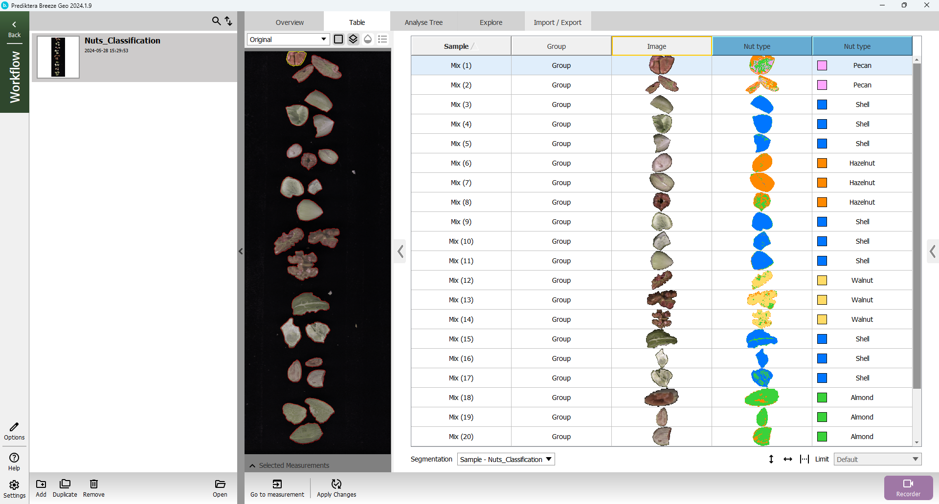
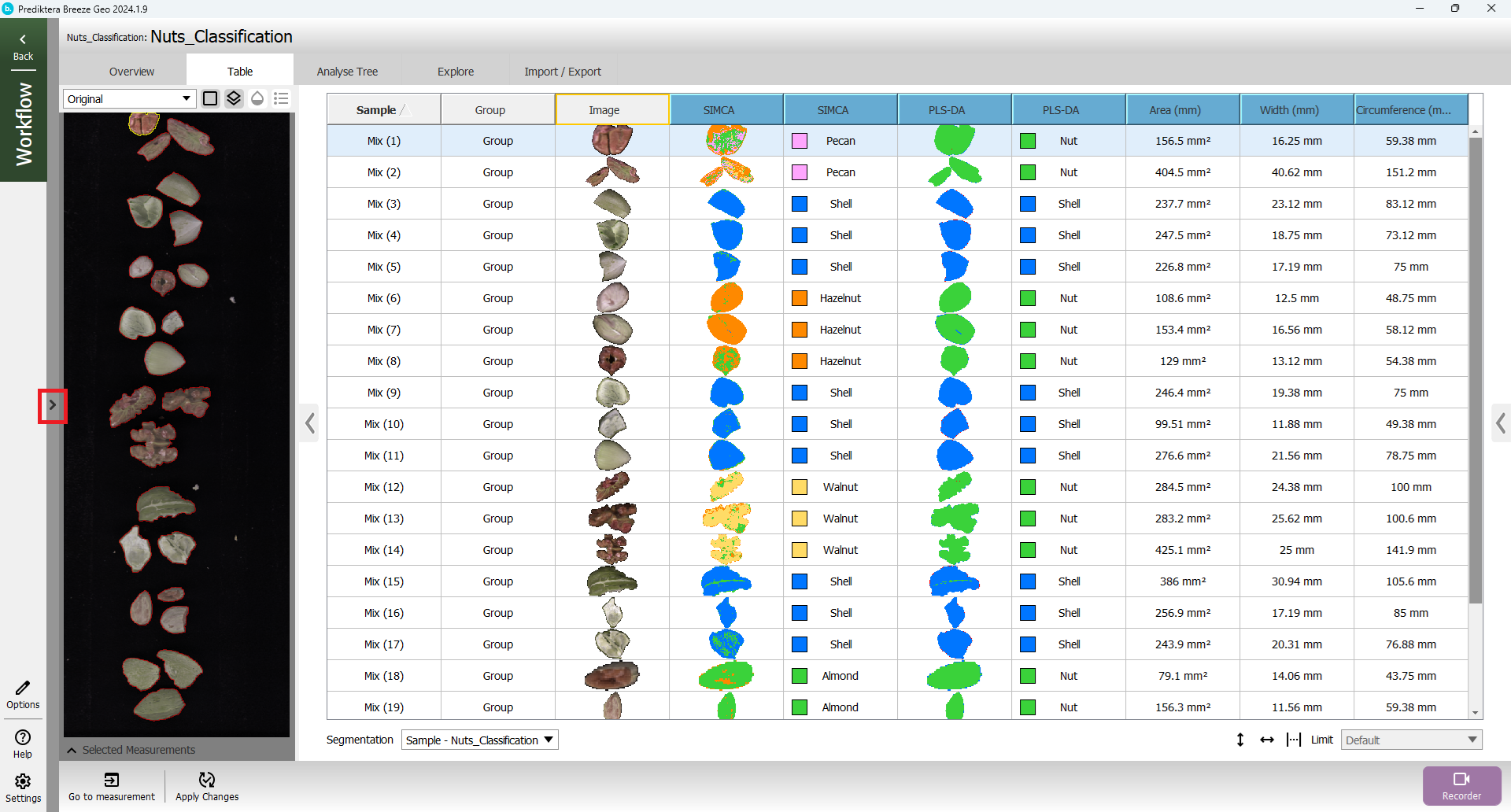
Open the Table view and then select Apply Changes.

The Table should now have new columns for the SIMCA and PLS-DA models, as well as for the Area, Width, and Circumference descriptors you added. Depending on your selections in previous steps your model results may be different, but after updating, your table should look similar to this. You can scroll the table to the right to see all columns, or reduce the Table width to fit them all on your screen.
To make more room for the table you can also minimize the panel on the right by clicking on the chevron button.
Nice job! You have reached the end of step 2 of the “Classification of Nuts” tutorial. See step 3 at: