Breeze can use a wide range of generic and specific Machine learning algorithms. Breeze can also import models created in other Machine learning frameworks which can export the models to ONNX format.
Before doing this tutorial, first, do the tutorial: Classification of nuts step 2
In this tutorial, you will create a Representative spectrum to expand on the existing data. Train a machine-learning algorithm to perform classification using the Auto evaluation mode to have Breeze select and train the most suitable algorithm. Inspect and fine-tune the model, and finally have a ready-to-run real-time classification workflow.
Steps included in the tutorial
Create representative spectrum
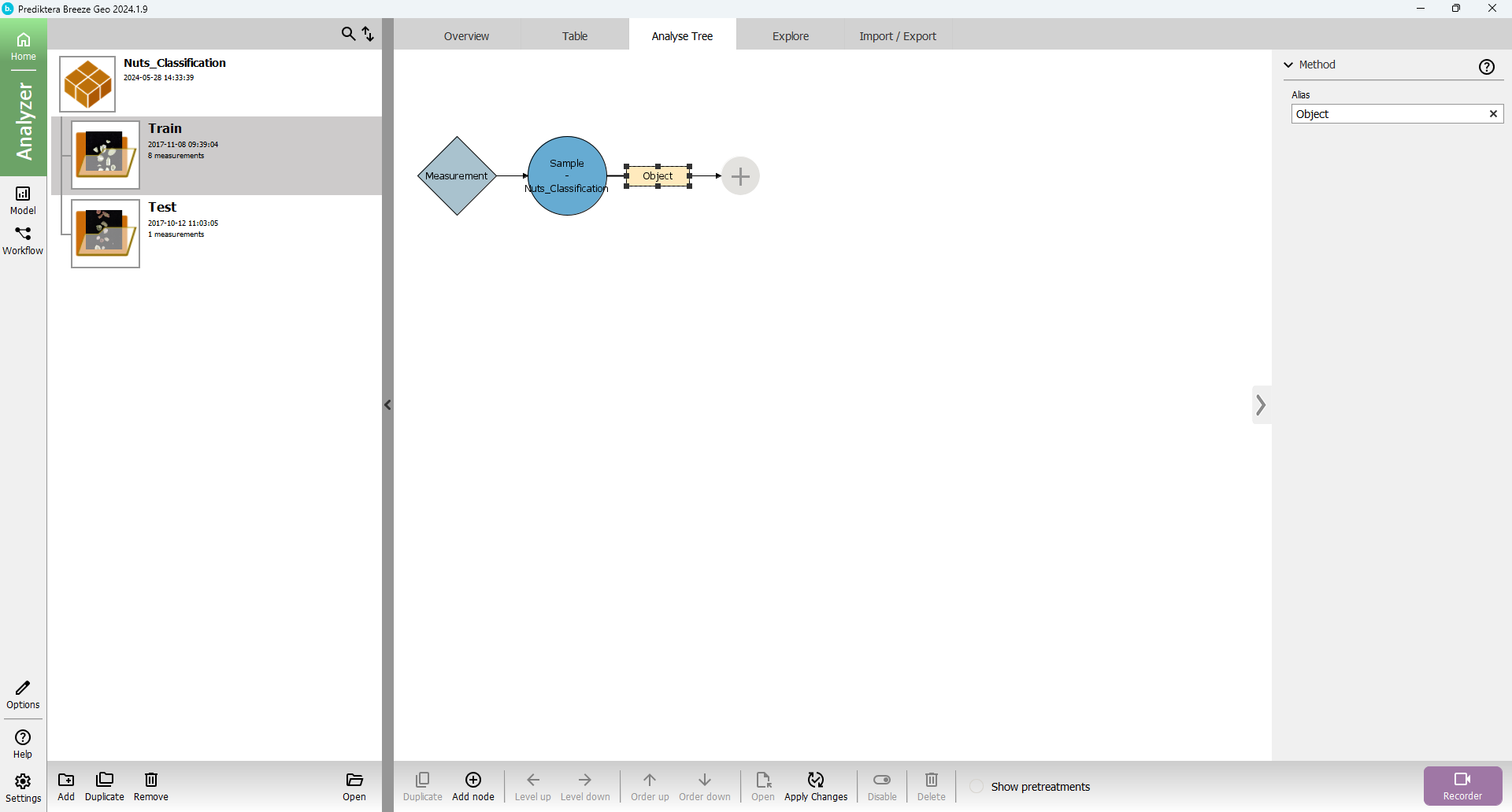
Open the project for the Classification of Nuts step 2 tutorial that you have previously done. In the group level open the Analyse Tree tab and add a new node after the segmentation object node by selecting the Object node and then clicking the plus sign.
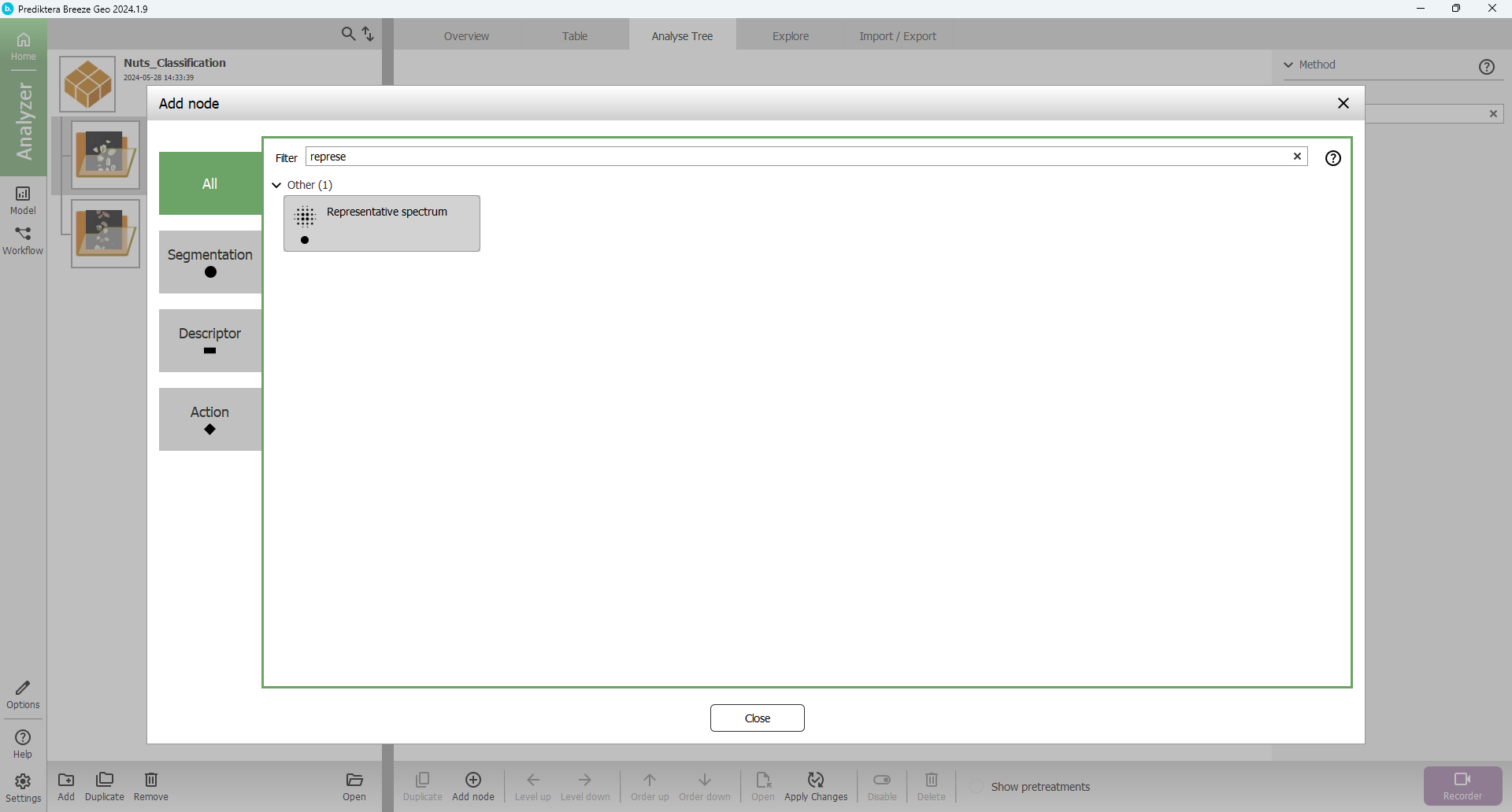
Select the Segmentation tab in the Add node window and select the Representative spectrum method.
Set Method to Random (Gaussian) for a random distribution with a Gaussian (normal) distribution.
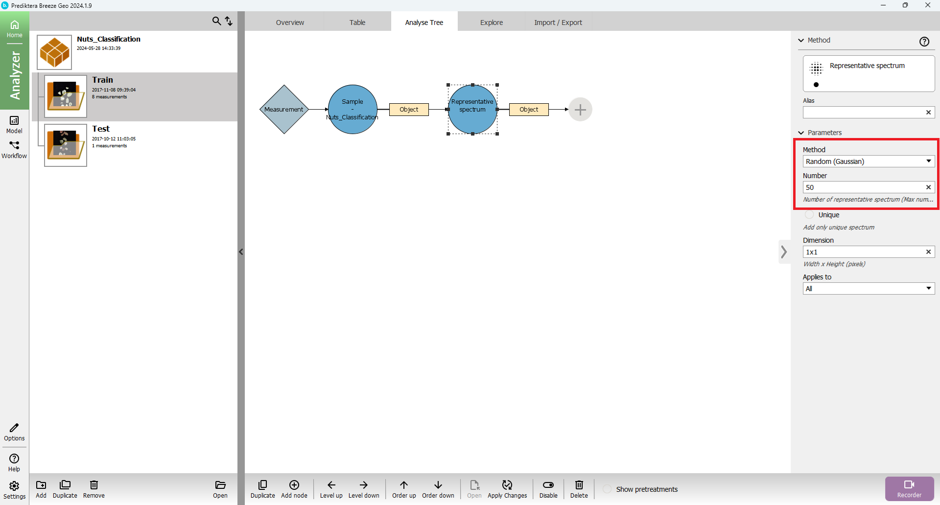
Set Number to 50 for a total of 50 pixels to be included from each object using the random Gaussian distribution. Set Unique to True so no pixels are repeated even if all pixels in the object have already been selected.
Press Apply changes to apply the new segmentation step.
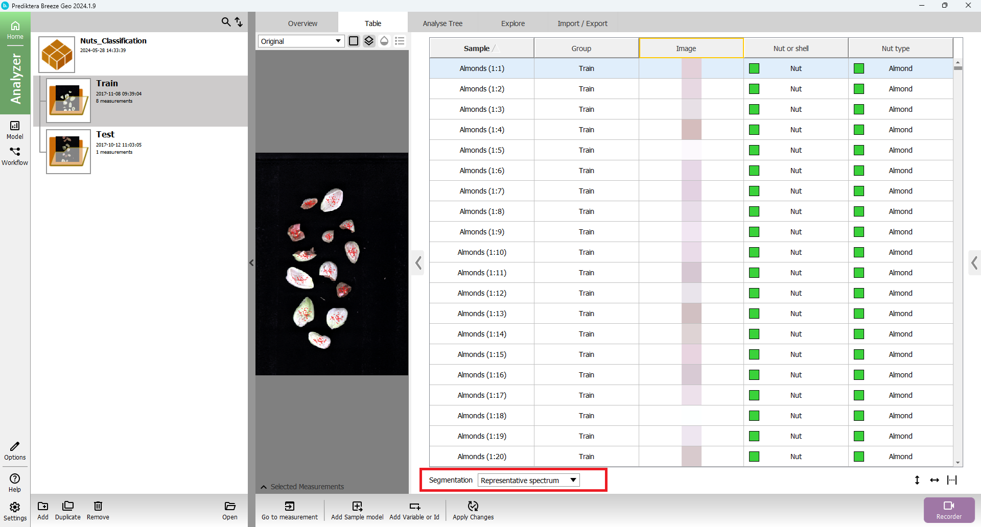
Open Table tab and select Representative spectrum in the Segmentation drop-down menu under the table. In the image on the left of the screen, you see that 50 pixels have been selected from each object.
Go to the Model view.
Create a Machine Learning model
Select Add and create a new Classification model selecting the method Machine Learning.
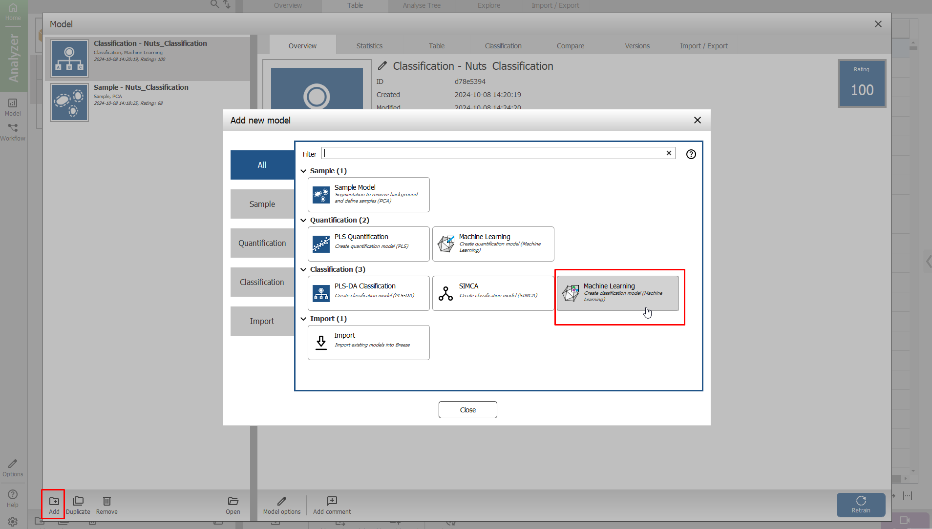
Use the suggested default model name and click Ok.
Select the newly created Segmentation Representative spectrum and Nut type as the variables to classify and click Next.
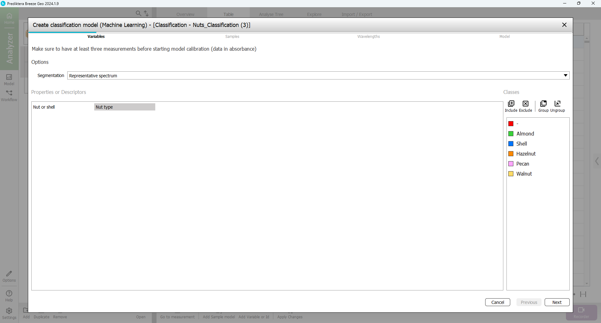
Click Next.
Here is now a list of all pixels that have been segmented out. You will use some of them as a training set and some as the test set. Scroll the list to the right so you can see the Group column. Select all the rows that are in the Group Test (select the first Test sample, hold down shift on your keyboard, and then scroll down to the last Test sample in the list and then click on it to select all samples in the Test group)
Select the Test button.
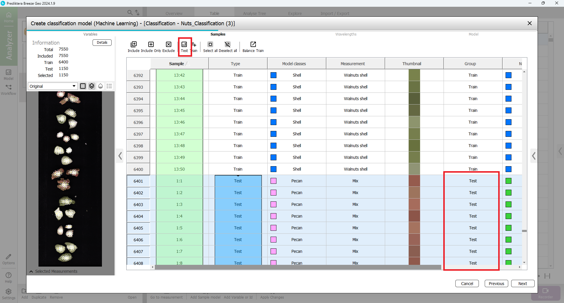
If you scroll to the left again you will see in the Type column that these samples are now selected as Test and the rest are Train.
Click Next to inspect which wavelengths will be used in the model.
Check the Show SNR checkbox to view the Signal-to-noise ratio. Order the SNR values in ascending order (least Signal-to-noise ratio) by clicking on the column heading, and select the wavelengths with SNR values below 1.6. Exclude them by selecting Exclude.
Finally check the SNV (Standard Normal Variate correction) (see Pretreatments | SNV (Standard Normal Variate correction) for more information).
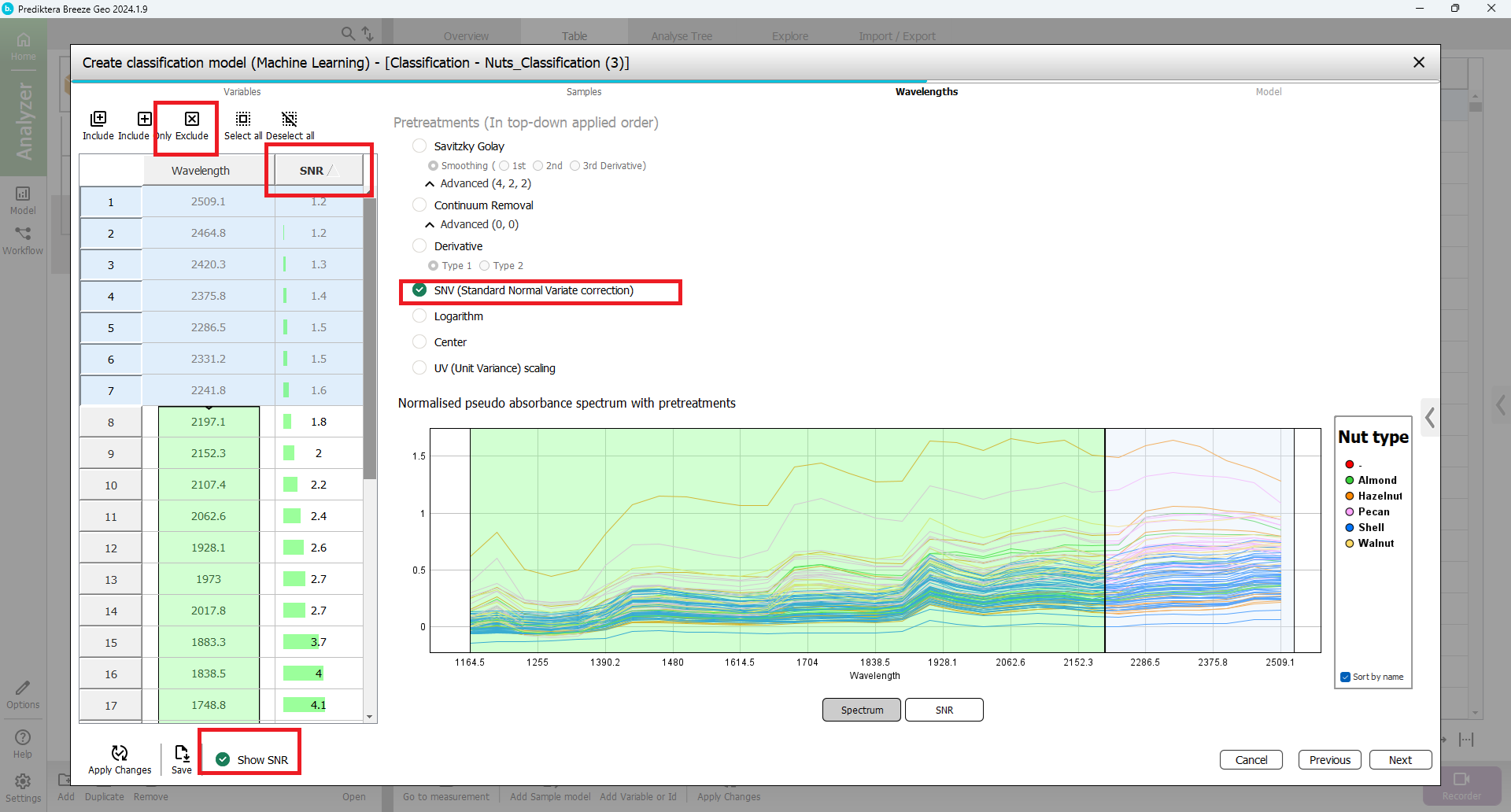
Click Next to accept the selections.
In the Model step of the wizard, set the training Time to 120 (seconds) and the Algorithm to Auto (default). Then click Train to have Breeze perform an automatic evaluation of the training data using cross-validation to find the best algorithm.
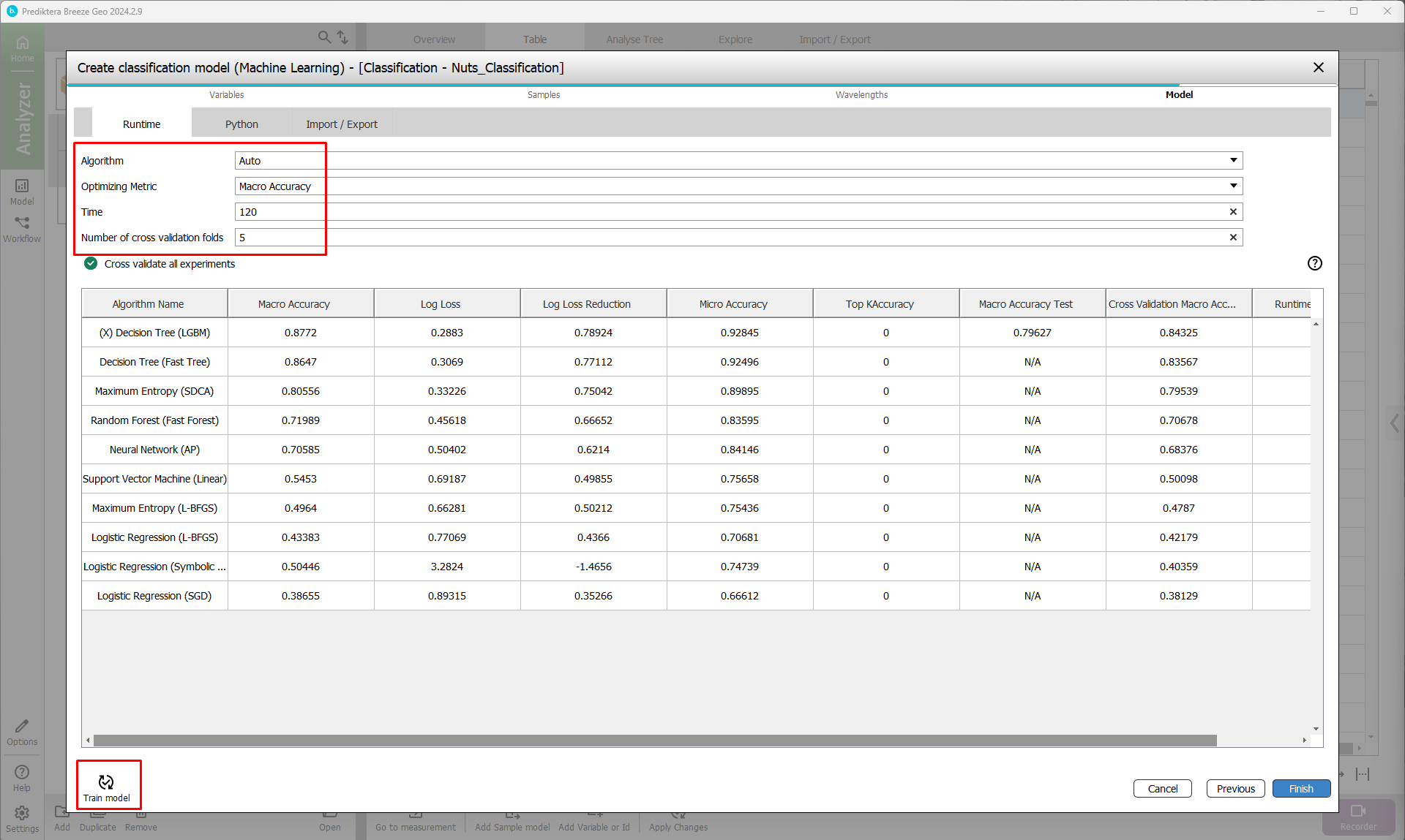
The resulting table is sorted in descending order of performance. The algorithm on the top has the highest accuracy and will be used for the model. Click Finish to accept the result and create a model of the best-performing algorithm.
Click the Workflow button in the sidebar to the left.
Real-time predictions
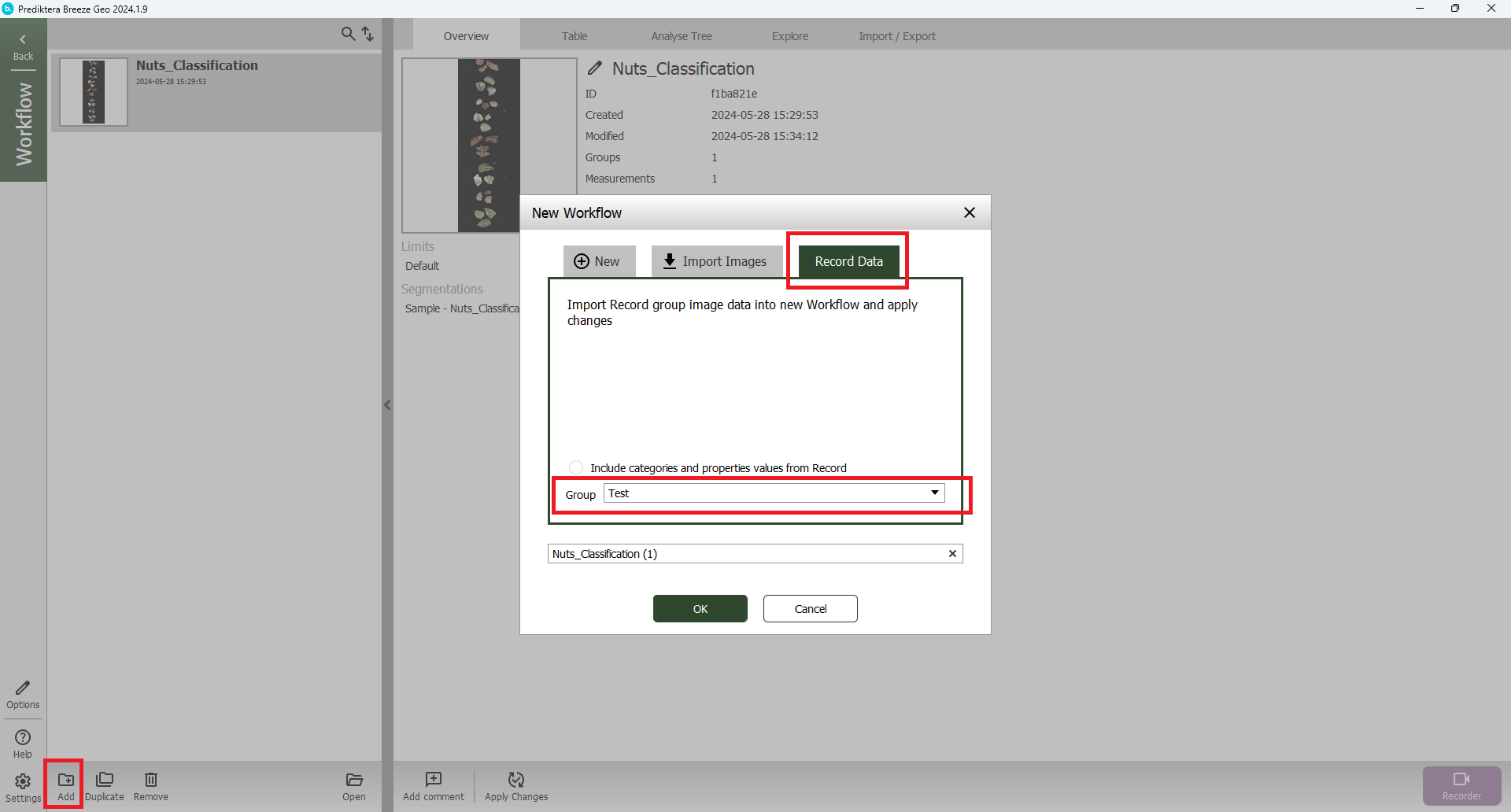
Click the Add button.
Select the Record data tab and make sure the Test group is selected, check the Include categories and properties values from Record option.
In the Table tab you may notice several columns, the first two are the actual (correct) classes that were added for each sample. The machine learning model only used the Nut type column for the training. Finally the last column is the results of the prediction from the Machine Learning classification model you created above (press Apply changes if you don’t seen any data in these columns).
To clear up space in the Table, you can right-click on the column header for the Nut or Shell column and delete it, since you won’t need it for this tutorial.
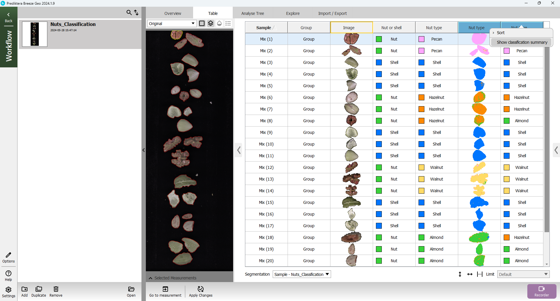
Inspect the results of the predicted Nut type compared to the actual one. Right-click on the prediction column Nut type and click Show classification summary.

The summary will indicate if there are any misclassifications of the objects. In this example, one Hazelnut is misclassified as an Almond (your results might vary slightly), and one Almond is missclassified as Hazelnut.
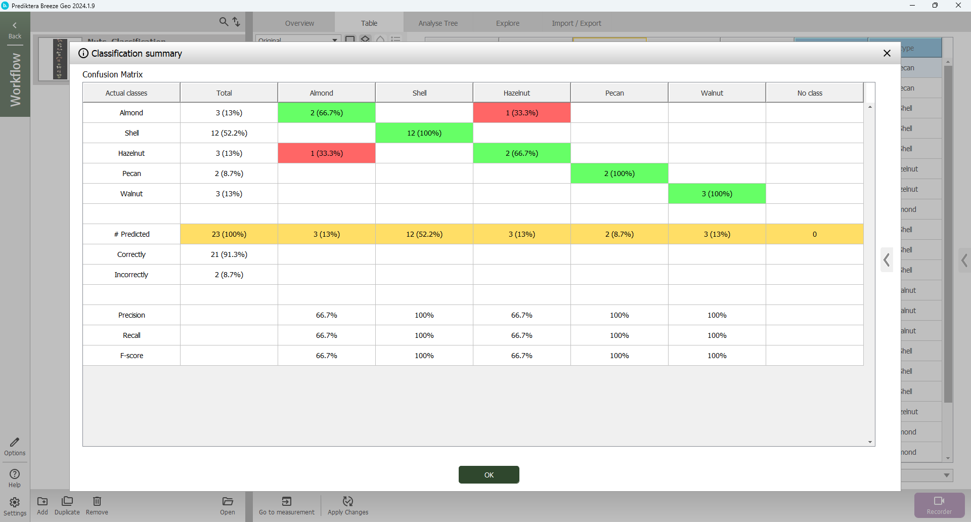
Close down the confusion matrix window.
When inspecting the Table you can see that for the misclassified nut (i.e. Hazelnut misclassified as Almond) the majority of the pixels are classified correctly, but the object classification is incorrect (this may not be the case in your model). The misclassification of the object in this case is due to the fact that the prediction is done at an object-level using the object's average spectrum, while the training data you used was based on 50 pixels from each object.
To remedy this you can change to object classification method. Switch to the Analyse Tree tab and select the classification node. Change the model Classification type from Object average spectrum to Pixels class majority. This will classify the object based on the majority class of the pixels.
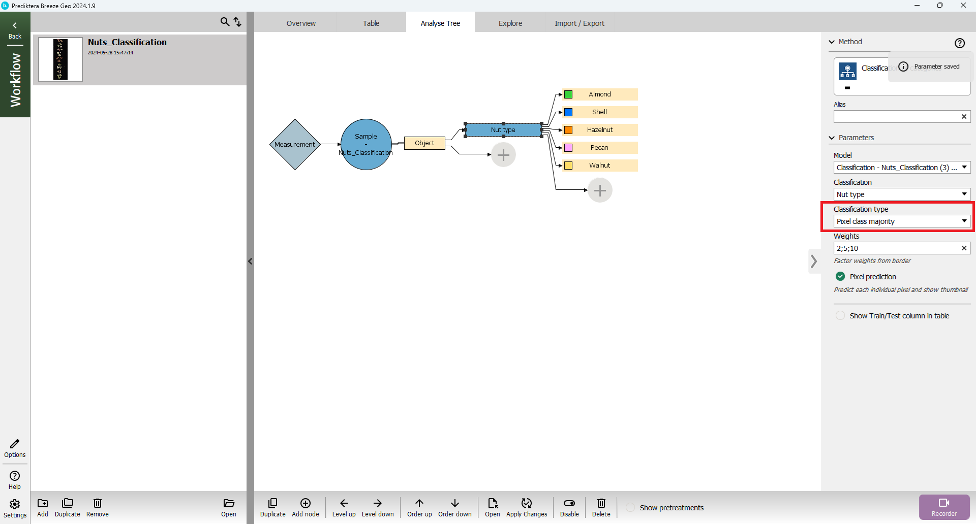
You can keep the default Weights (2;5;10)
Which are the weight of the pixels as such:
-
2 - closest to the edge of the object
-
5 - second closest to the edge of the object
-
10 - the center of the object.
The default weight implies the center of the object is most representative of the spectrum while the edge is less so (entering the value 1 would make all pixels equally important).
For full details, see Classification of categories.
Click Apply Changes.

Now let’s inspect the Table to see if the samples are correctly classified.
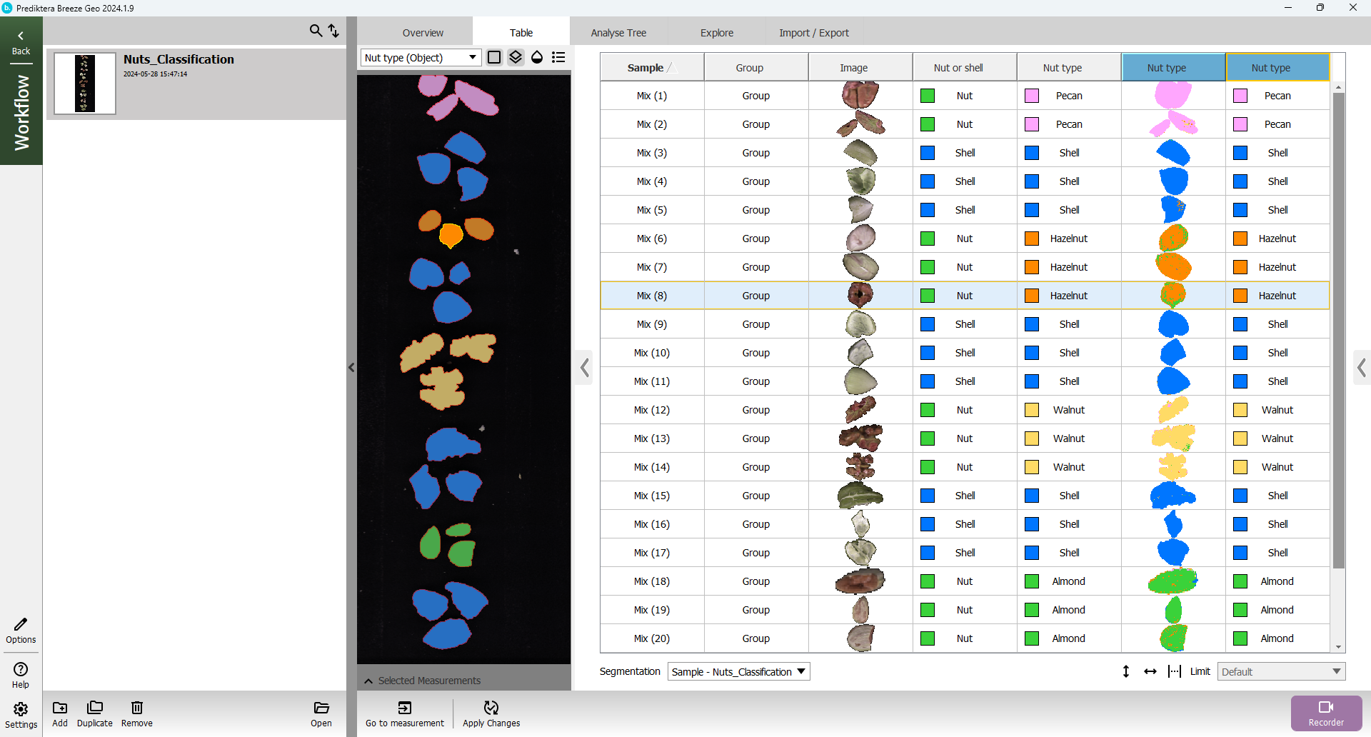
Right click on the header for Nut type and the select Show classification summary.
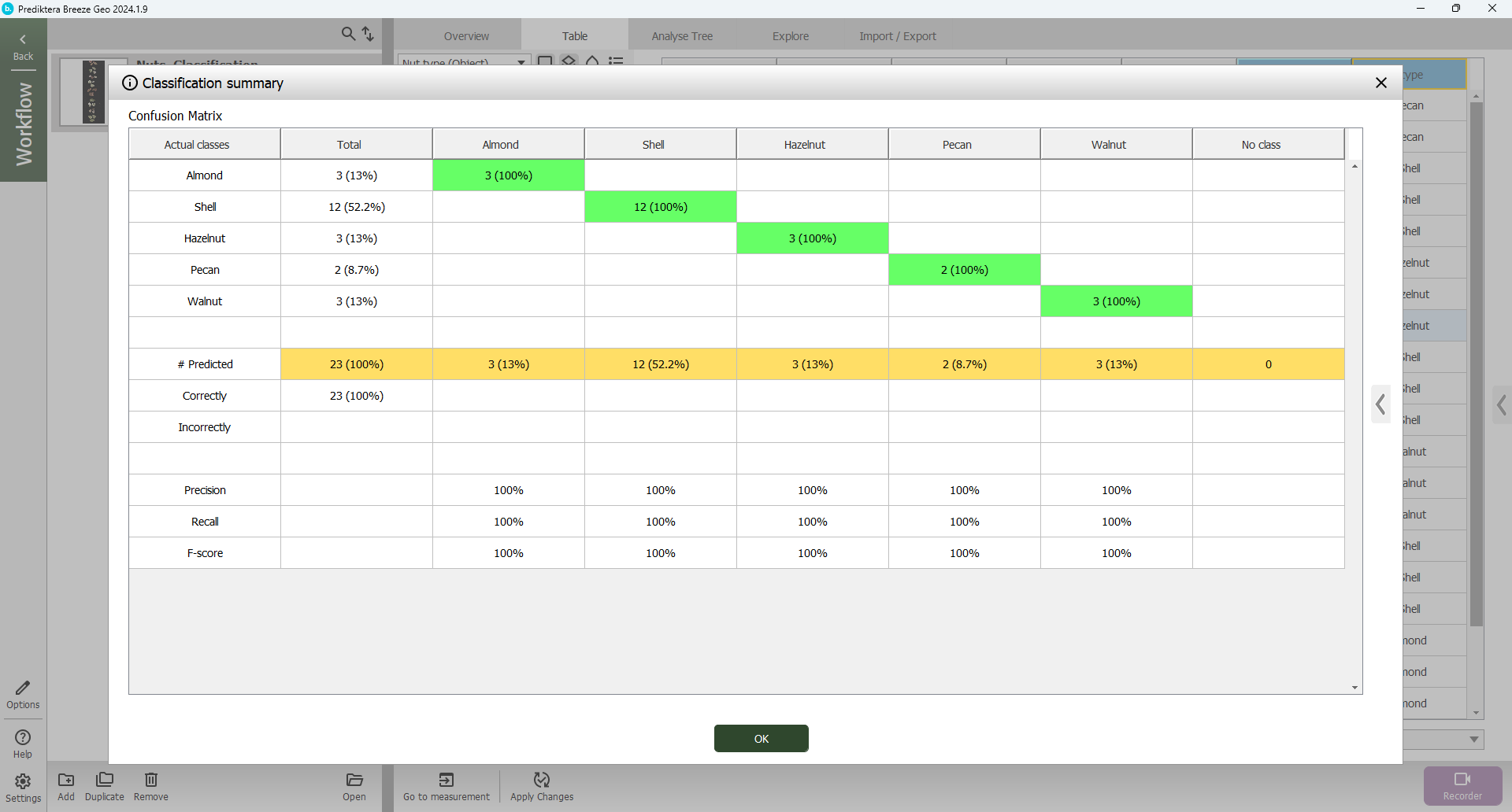
Your model should hopefully also receive a perfect object classification.
The model classification is now ready for real-time predictions. To test this, click on Recorder and the same images used for training the model from the test set can be evaluated in a real-time scenario.

Select the existing groups or make a new group. Uncheck the Save image measurements and calculated descriptors option and select Parallel Measurement segmentation.
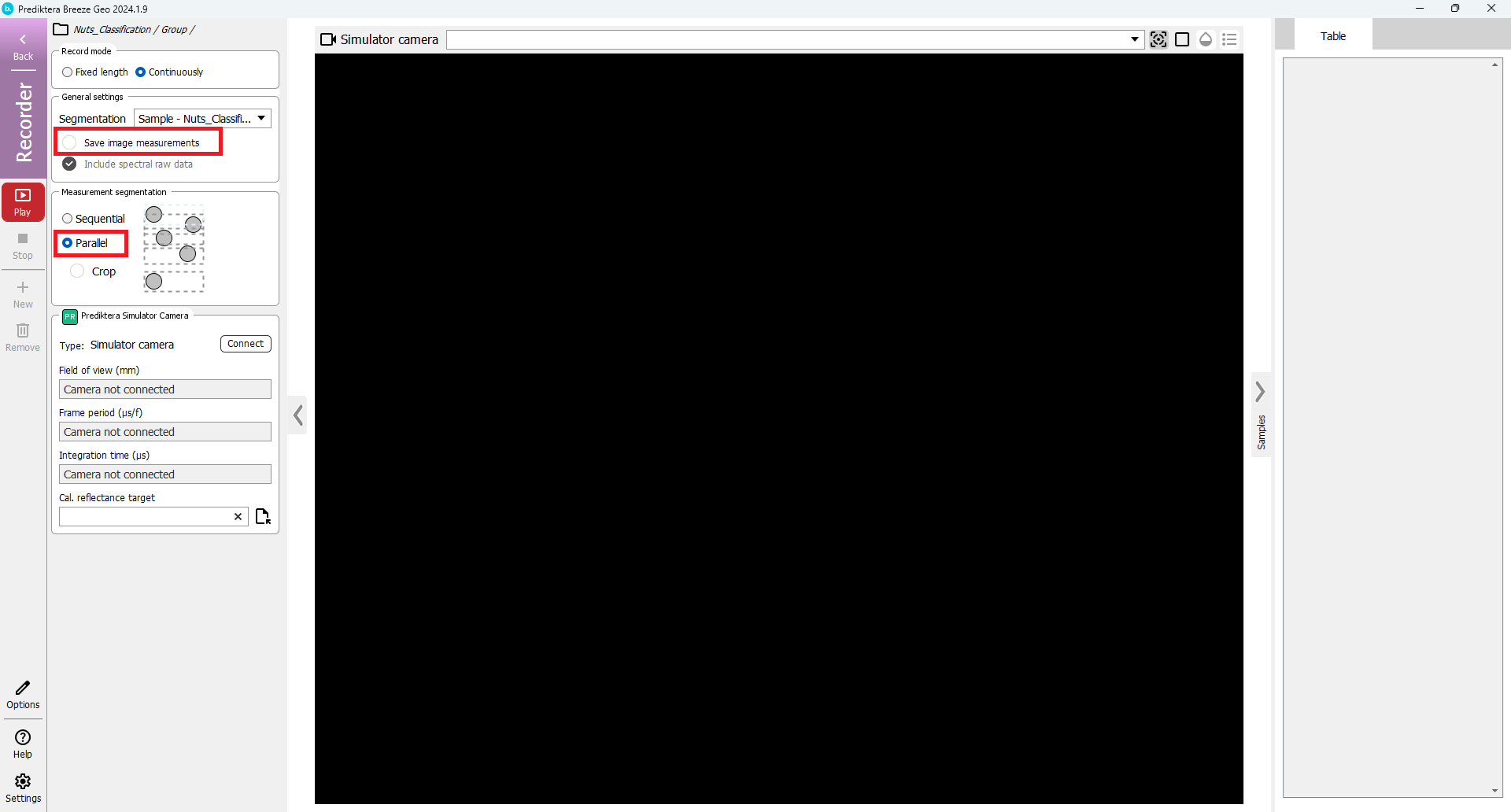
Click Play. You should see a wizard for the the white reference procedure. Press Take and then Record.
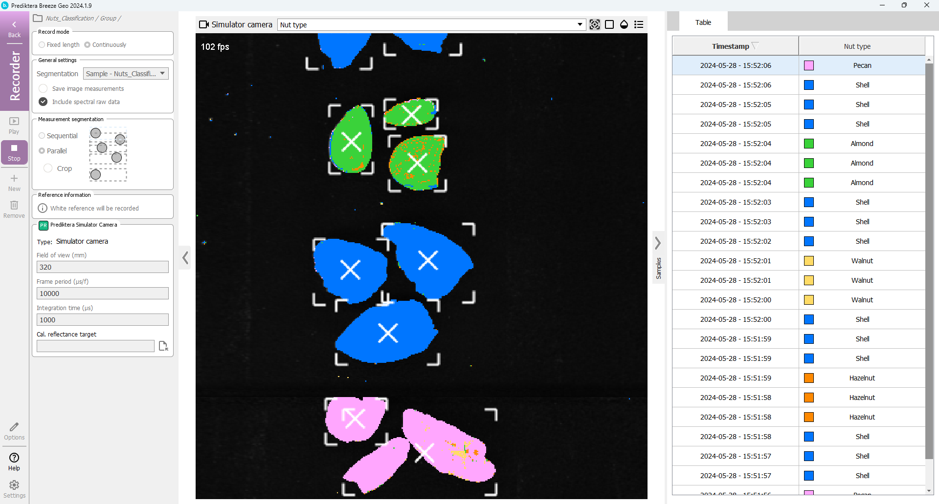
Good job! Watch the classified nuts roll by and receive a perfect classification score. Click Finish to stop the predictions.