Breeze Geo Logging and classifying of the drill core

The training data

The training data consists of three images containing three different core boxes. The spectral acquisition was carried out using a HySpex SWIR-384 camera, with a 930-2500nm spectral range at the Colorado School of Mines core scanning. The core boxes were placed on a moving stage under the stationary camera and broadband halogen lamps were used as illumination sources.

In this tutorial you will learn how to:

1. Use the core logging tool in Breeze Geo to log the core

2. How to segment the core based on the core logging

3. Create 10-centimeter intervals throughout the boxes

4. Classify the segmented core using the MICA expert system

5. Apply Dominant minerals and Pixel by given class

6. Export the result

Download and import tutorial image data

Start Breeze

Press “Tutorial” and choose “Drill Core Logging and Classification” in the dropdown menu and press OK

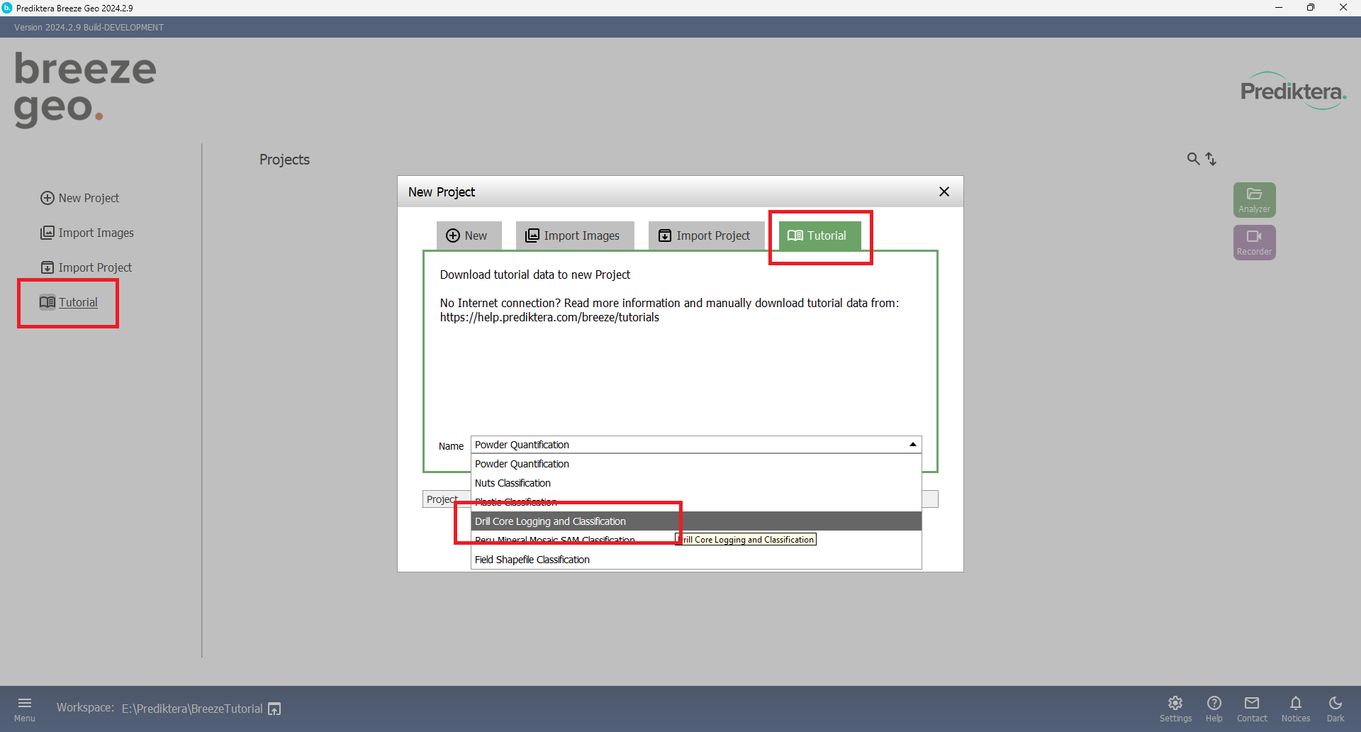
After the tutorial data is downloaded a project will appear in Breeze Geo

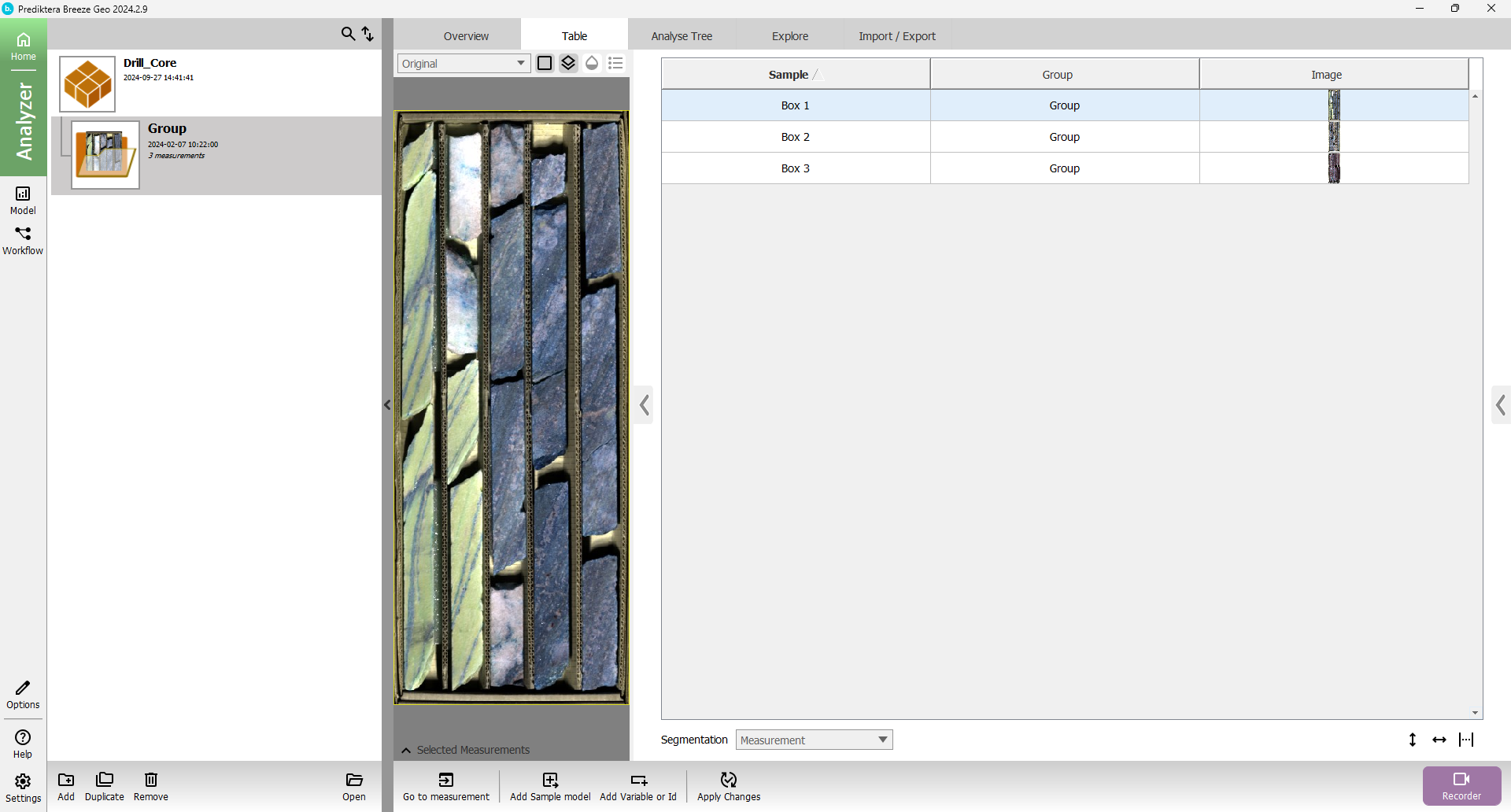
The project you downloaded is called “Drill_Core”. The images of the core boxes in the study can be seen in the table. You can press the images in the table to see the different pseudo-RGB images for the different boxes.

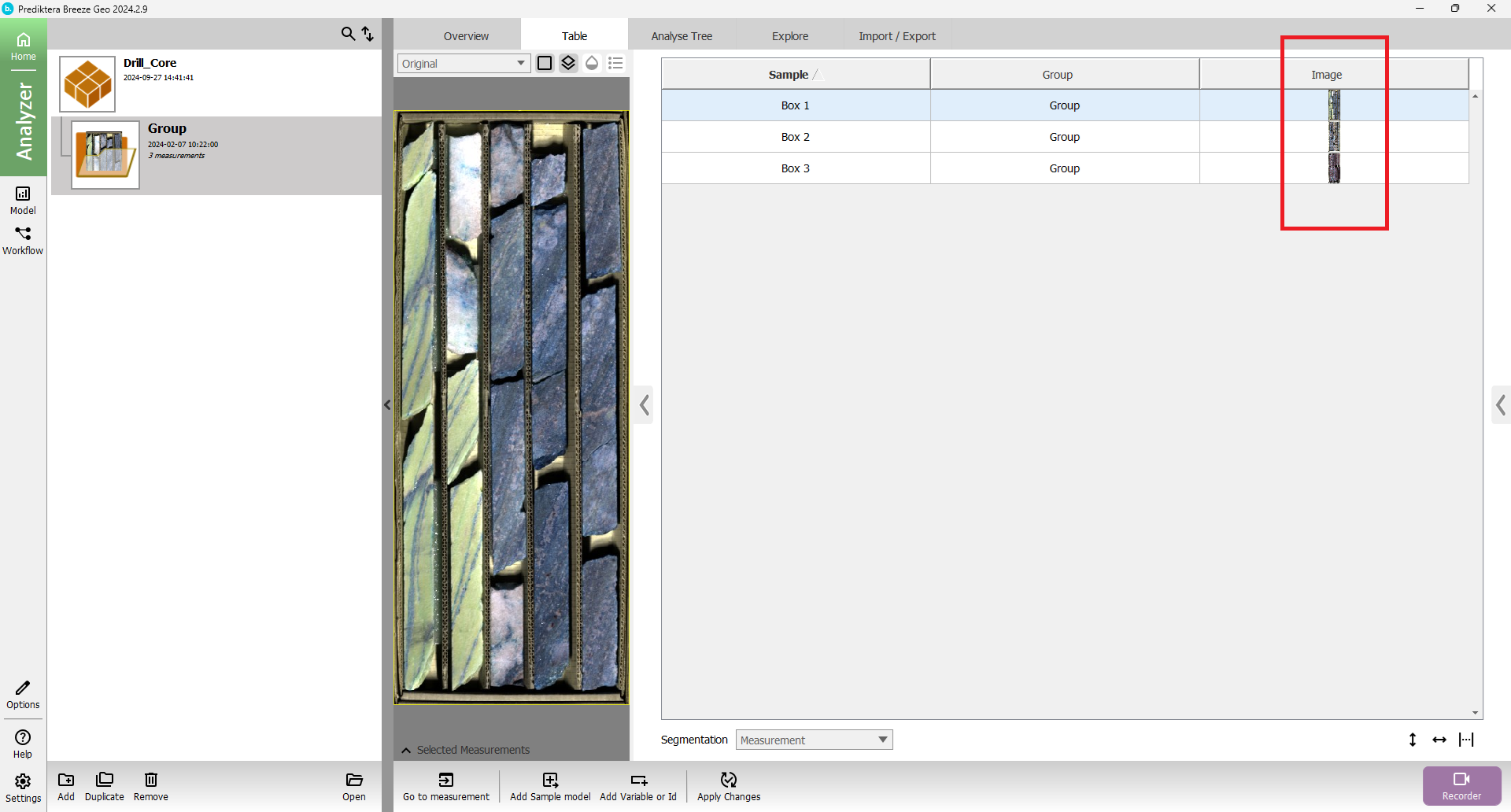
Click on the “Open” button to open the study or double-click on the study name in the left column.

You are now in the measurement level and can see the three measurements included in the group.

View spectra in pixel explore

Click on the “Pixel Explore” tab. In Pixel Explore you can browse at the spectra in the images. Spectra can be viewed by manually selecting an area using "Free", "Ellipse" or "Rectangle" or use "Pixel" to view one spectrum at a time."

If you select an area larger than one pixel, you are viewing an average spectra of the area.

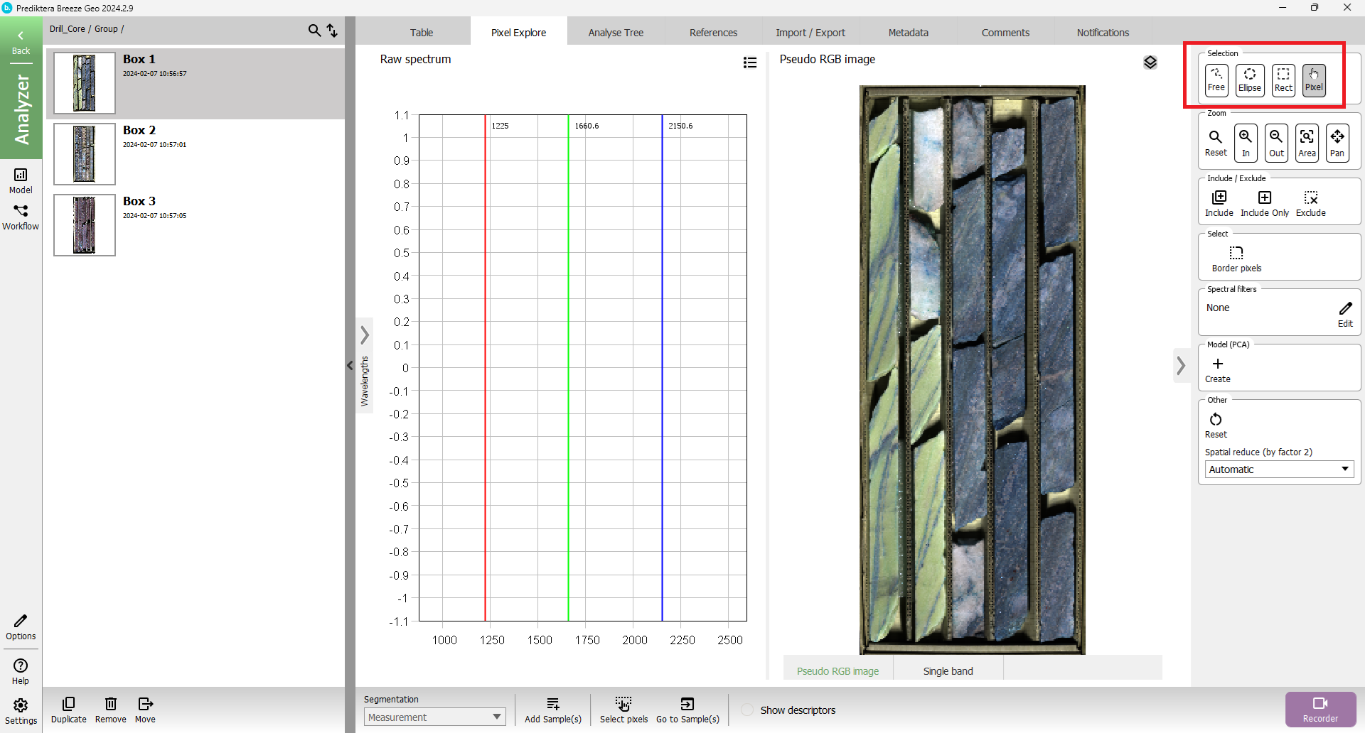
Select the pixel tool hover with your mouse over the pseudo-RGB image and left-click with your mouse over a pixel of interest. Do this at different parts of the images and you will see more spectrum appear in the spectrum plot. The spectrum shown represents the spectrum from the selected pixel.

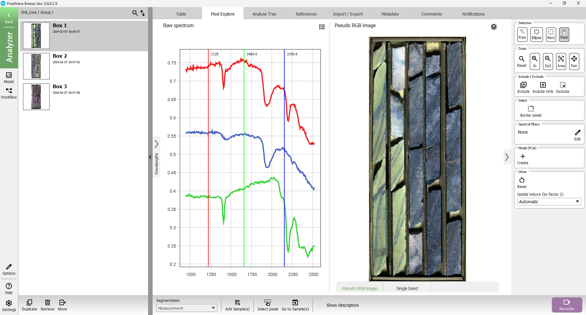
Feel free to select another image from the menu to the left and look at the spectrum for the other two images as well.

Enable depth registration

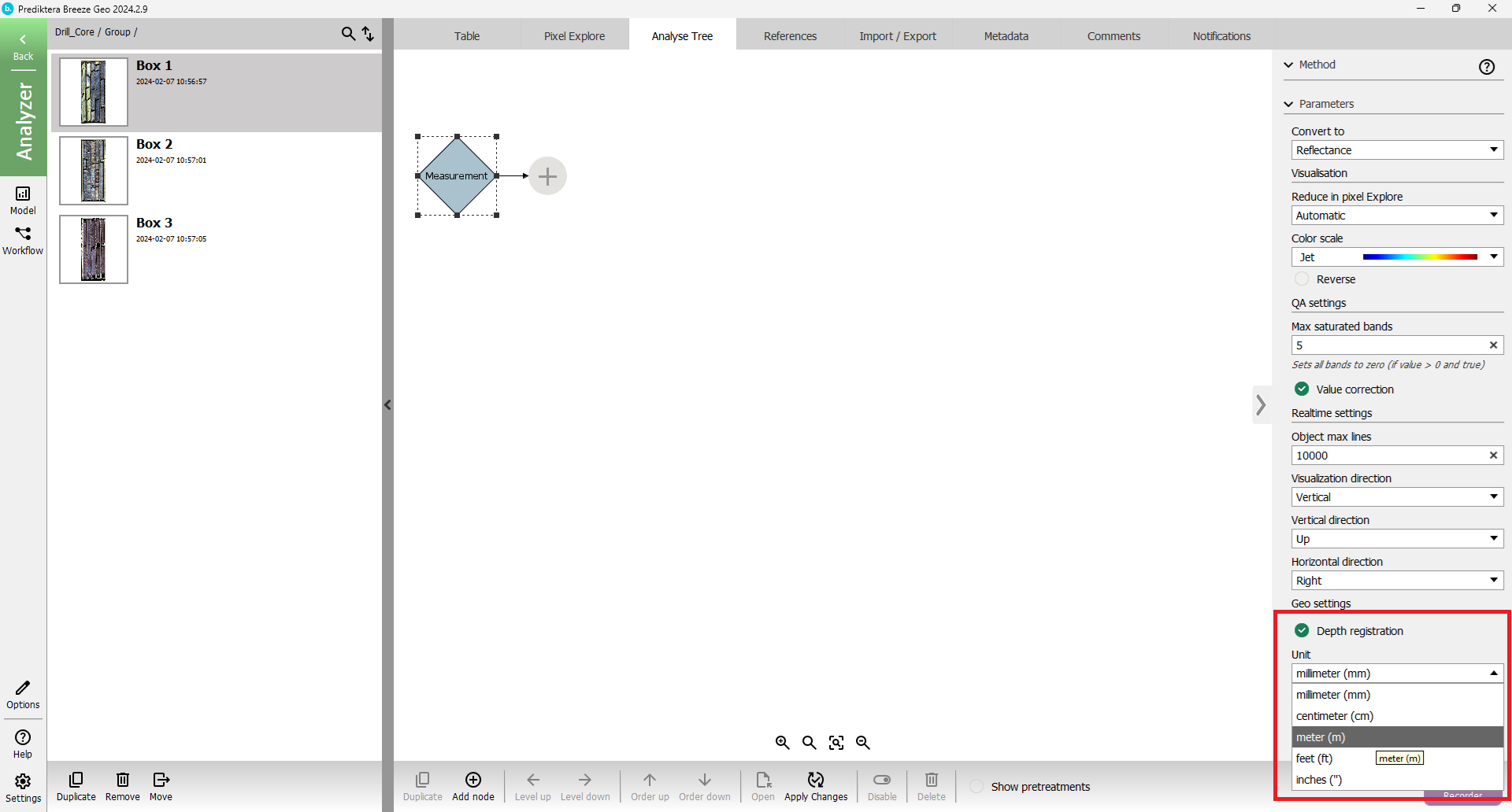
To enable the core logging tool, first need to go the “Analyse Tree” tab and left-click on the “Measurement” icon. In the menu to the right, check the “Depth registration” box. We will also change the “Unit” to meter (m), other unit options include feet (ft), inches (''), and millimeters (mm).

Press the “Back” button in the upper left corner to get back to the Group level and then double click the group to open the Measurement level again.

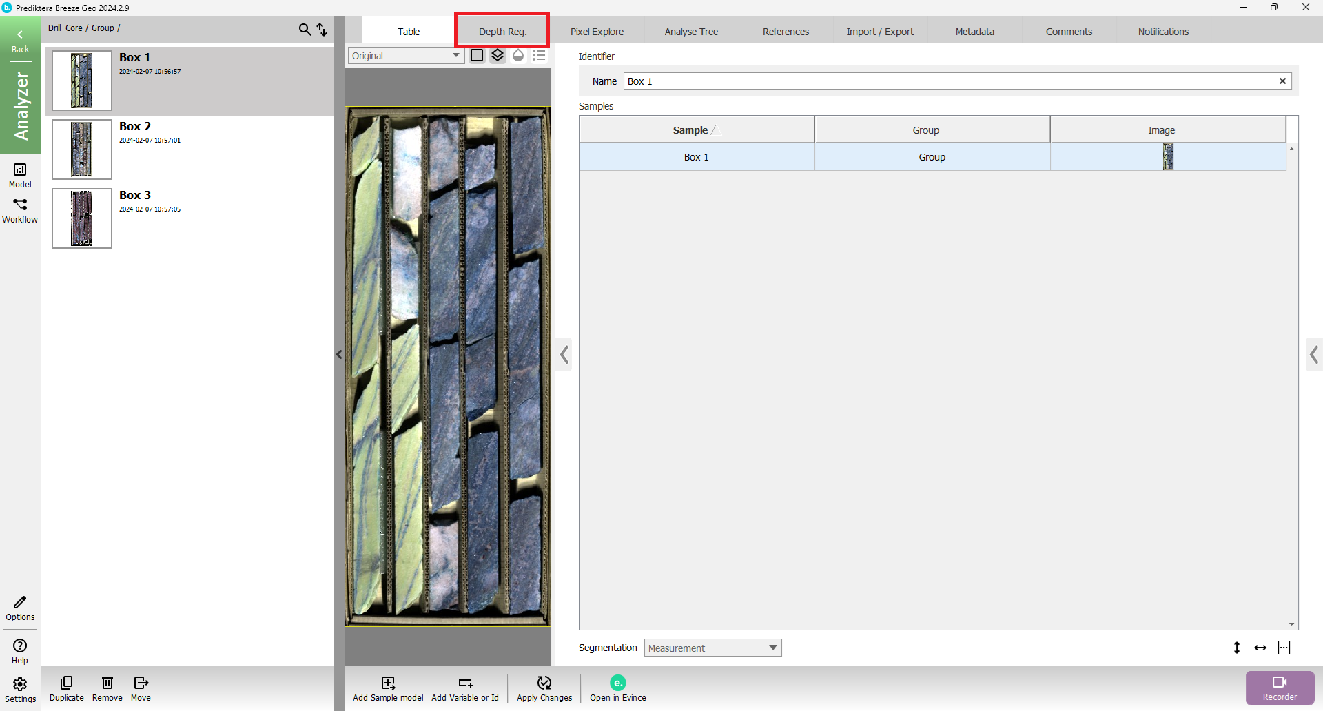
Executing the previous step will refresh the "Measurement" toolbar. A "Depth Reg." tab will now be included. Click the Depth Reg. tab.

Core logging

Start by pressing “Zoom out” until the whole box is visible.

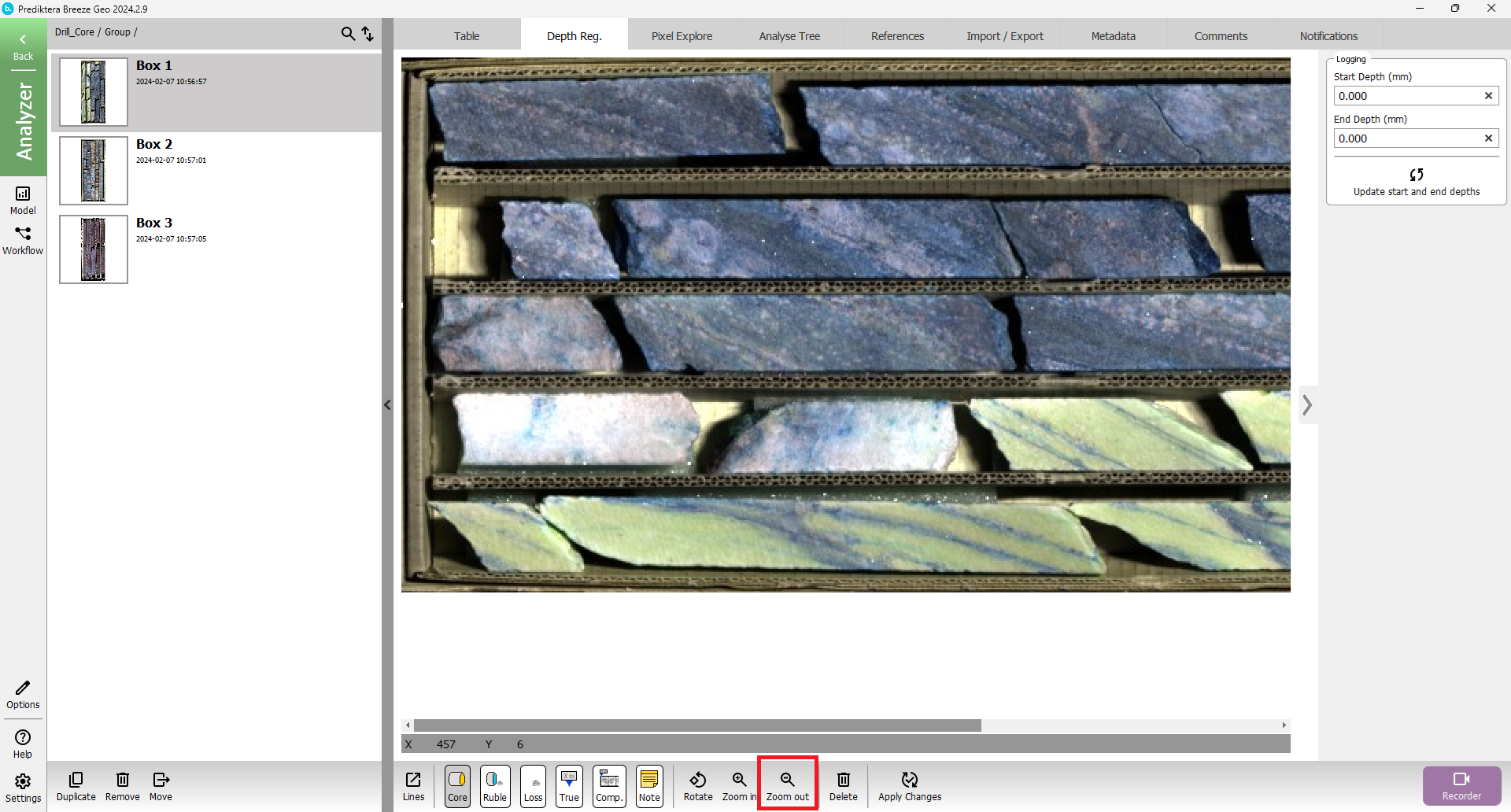
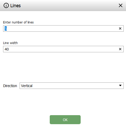
Then press the “Lines”, since the box has five compartments write 5 under “Enter number of lines” change the “Line width” to 40, and press “OK”.

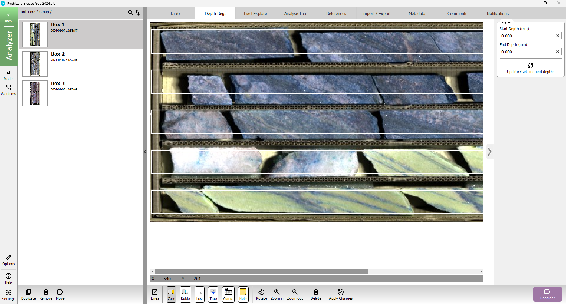
There will not be 5 white boxes on the core box image that are 40 pixels wide to mimic the width of the core.

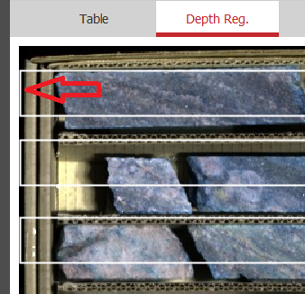
To adjust the position of the lines on the box, hover over the left or right edge of the white box and the mouse will change the icon to . Move the lines so the rectangular boxes cover the core. Make sure the “Core” option is selected (highlighted in blue).

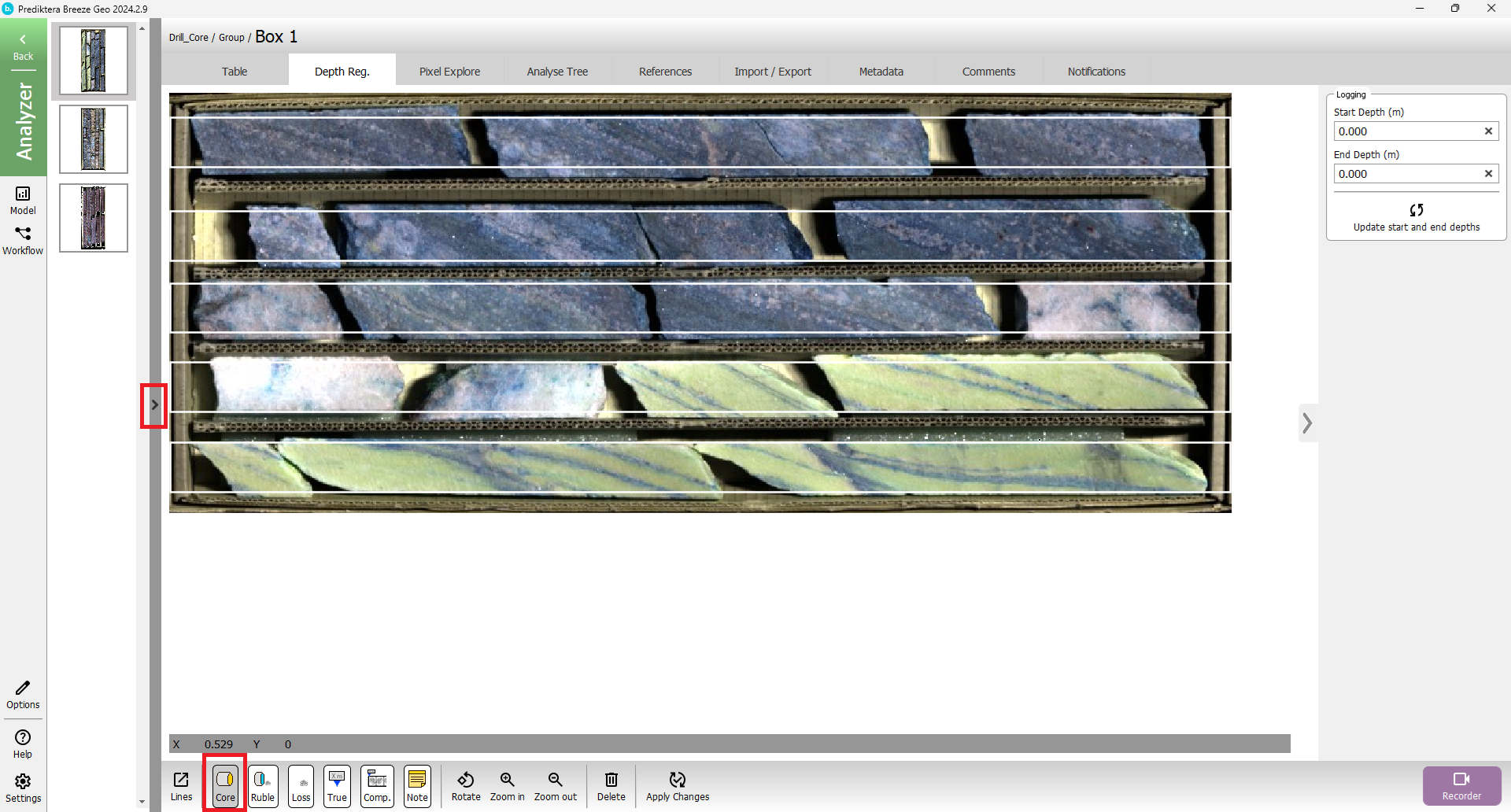
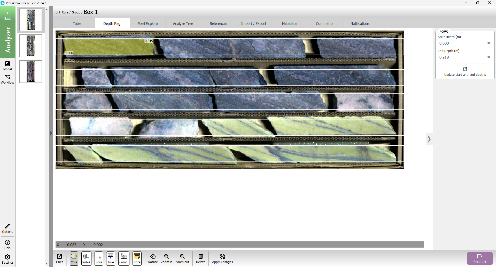
Now hover over the core and double-click using the left button on your mouse at the top left corner of the core box. If you drag your mouse toward the right you will see a yellow cover over the core. This is to highlight the logging of the core. you can also see the length of the logged part. The numbers are in the unit we selected previously and the length is calculated using the resolution of the camera. When you come to the crack of the core left-click once and the logging will stop. It should look something like this

Continue logging the core by double-clicking again. Continue doing this throughout the core box, at the end, you should have something like this.

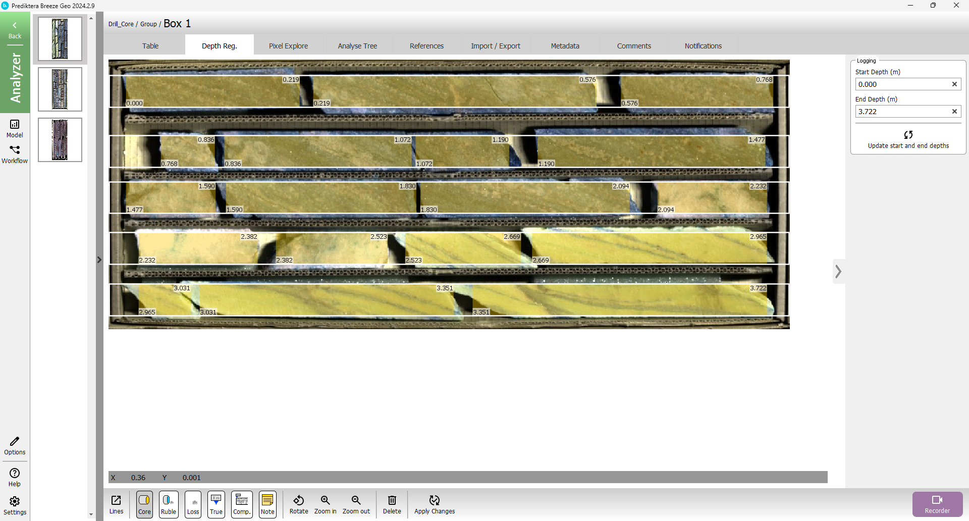
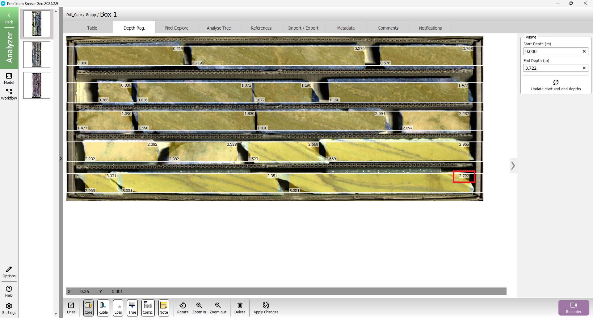
Note the end depth in the lower left corner. Here it is “3.722”

Press box 2 in the left menu and add the end depth of the first box in the “Start Depth” to the right. Then go through the same procedure under Core logging to log the core for both Box 2 and 3. A complete core logging of box 2 and box 3 should look like this

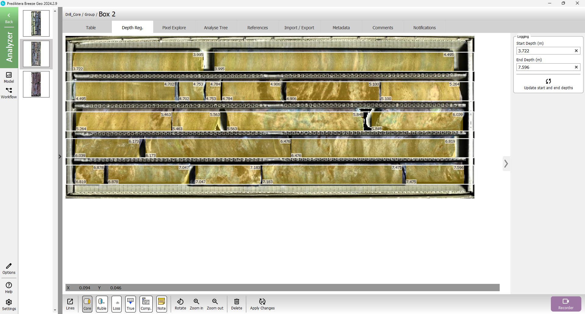
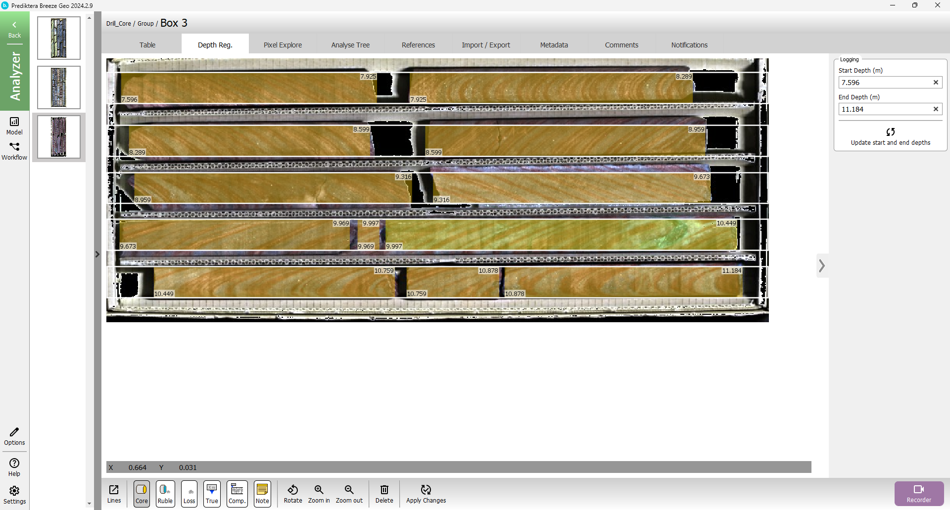
Segment and divide boxes into intervals.

When all the boxes are logged we can start segmenting and divide the core into intervals. Go to the “Analyse Tree” press the measurement icon and press the plus sign.

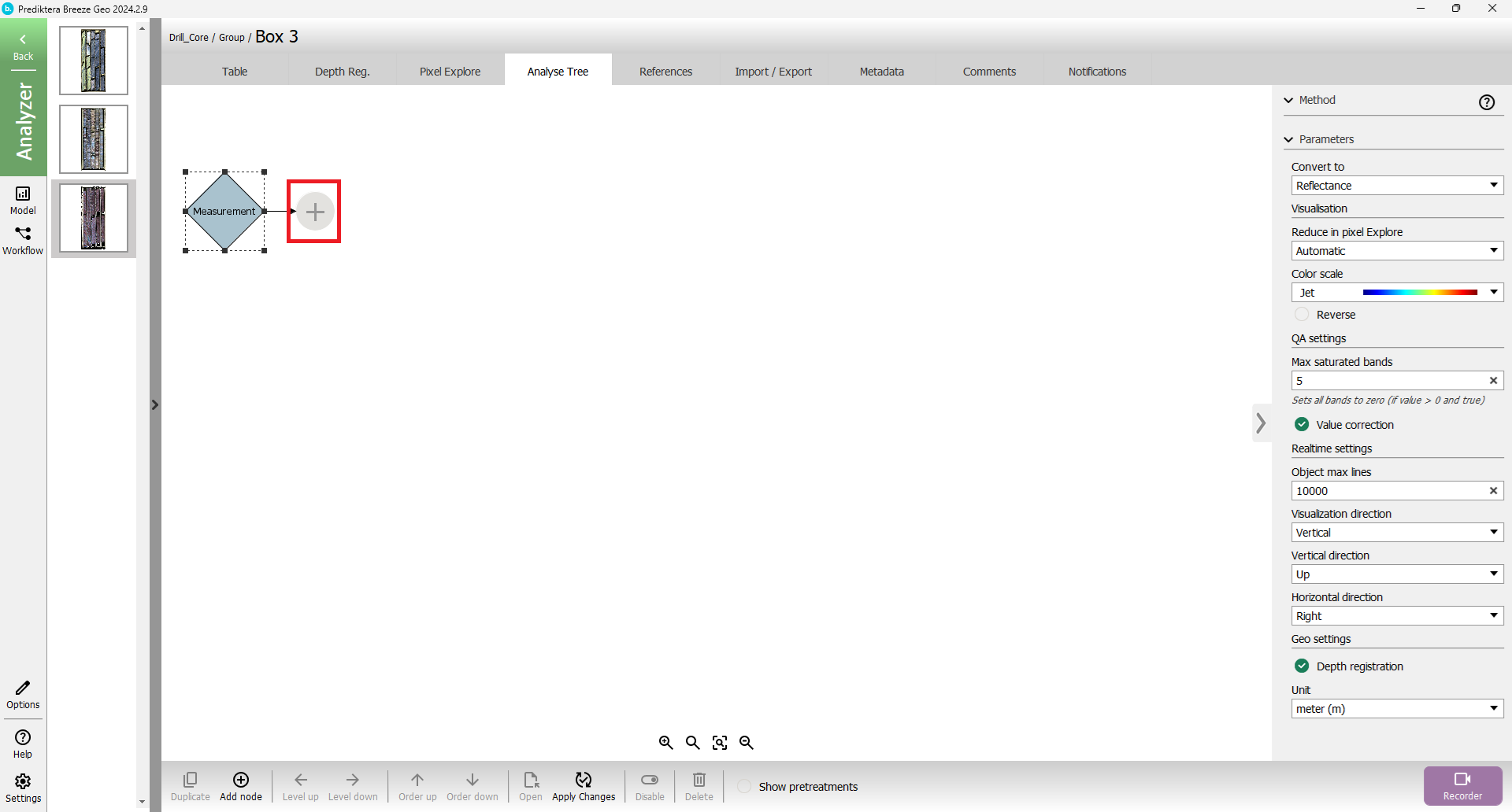
Add the segmentation “Depth registration” and change the merge from “None” to “All lines in box”.

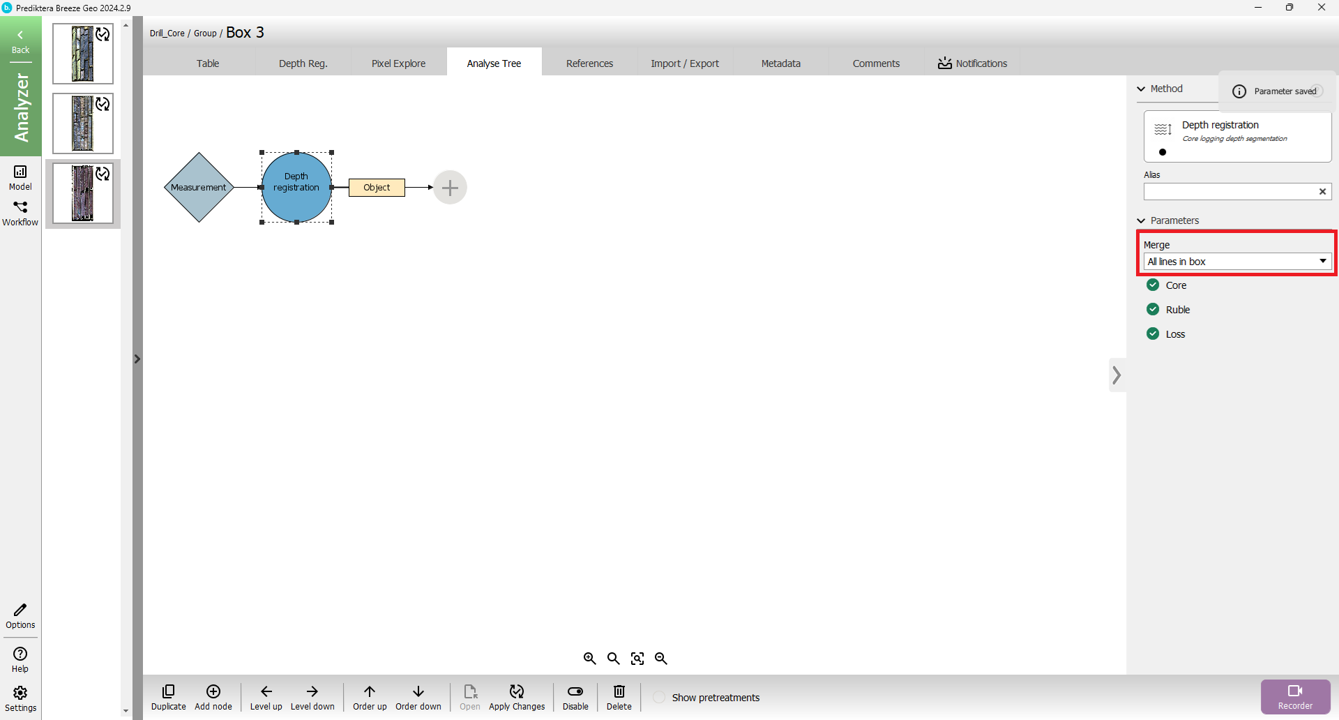
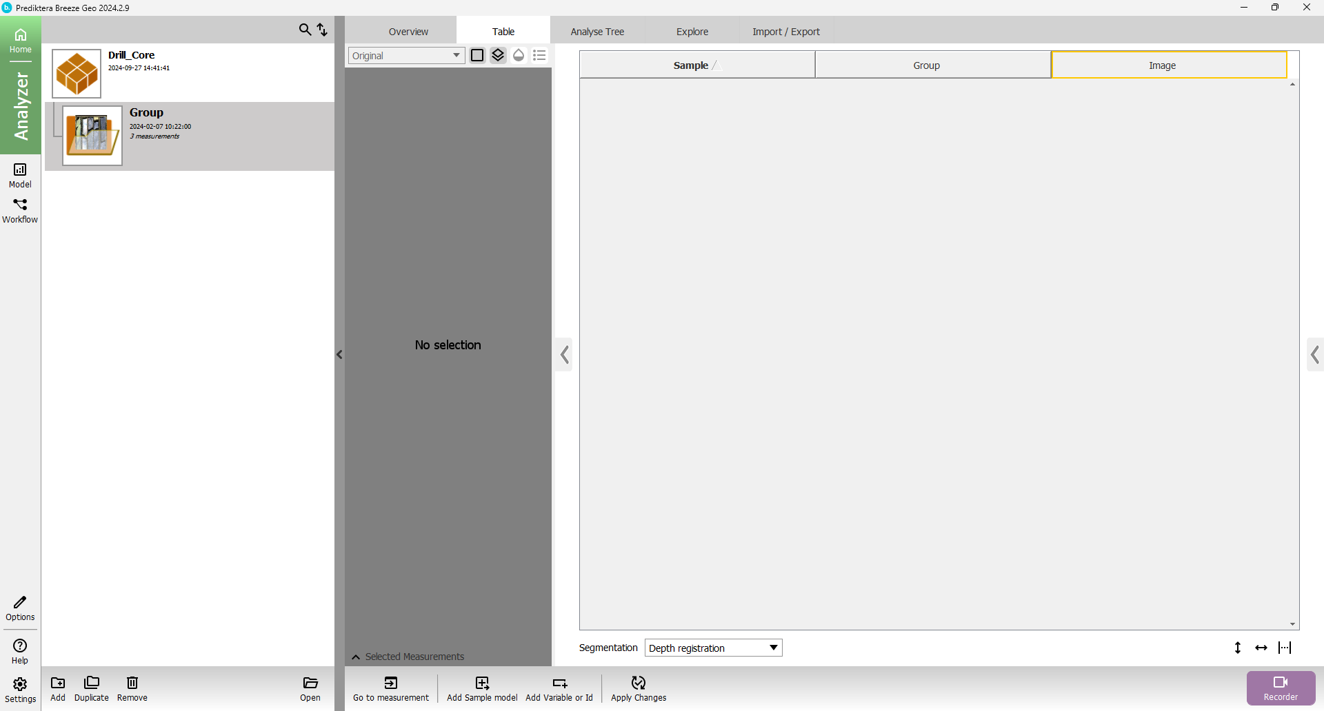
Press the “Back” button in the upper left corner to go back to the group level and then select the table view.

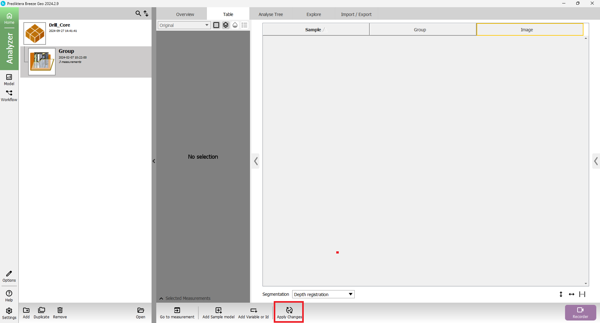
By pressing "Apply Changes" in the Group level, the new Analyse Tree will be applied to all of the measurements in the group.

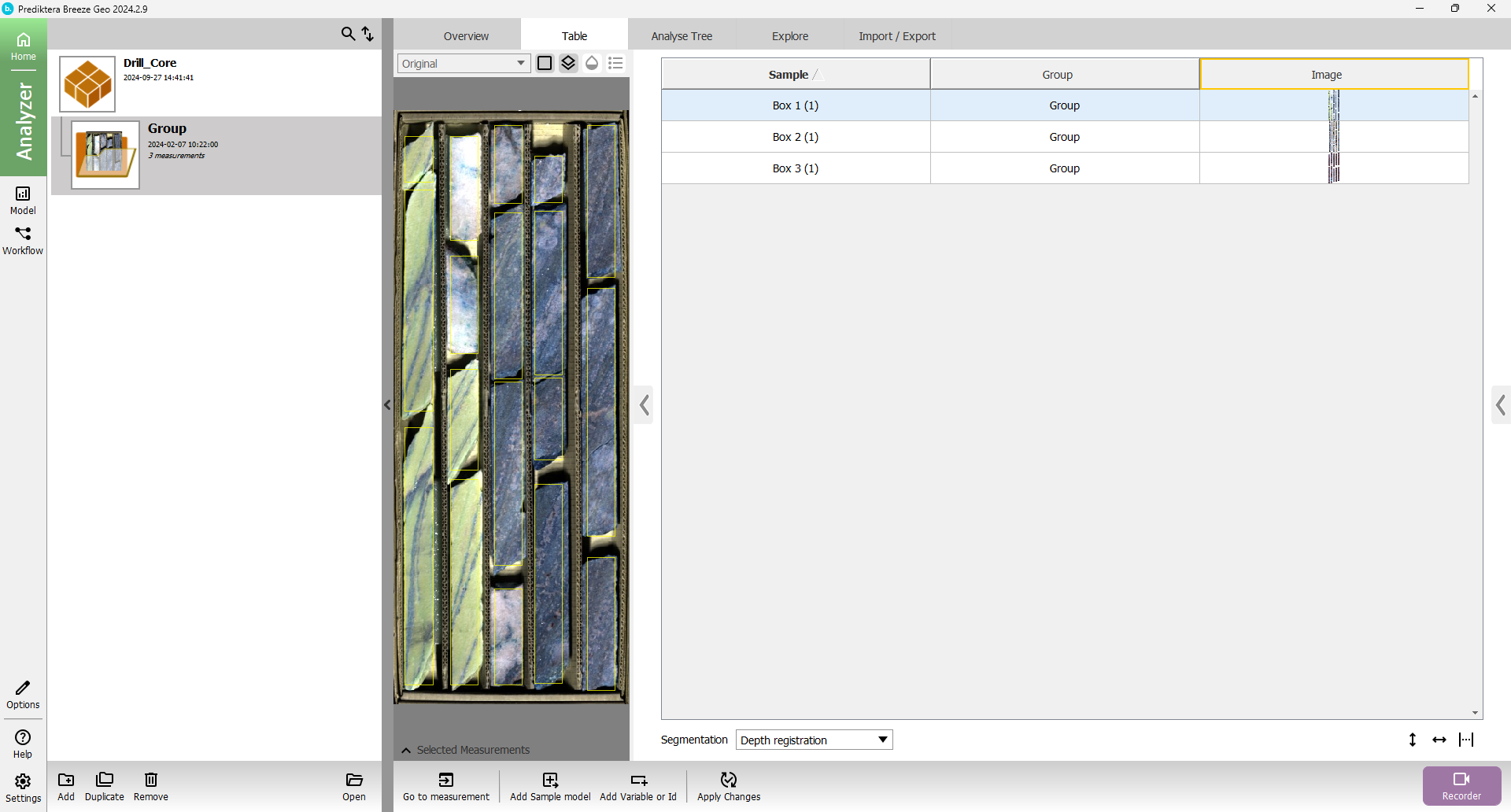
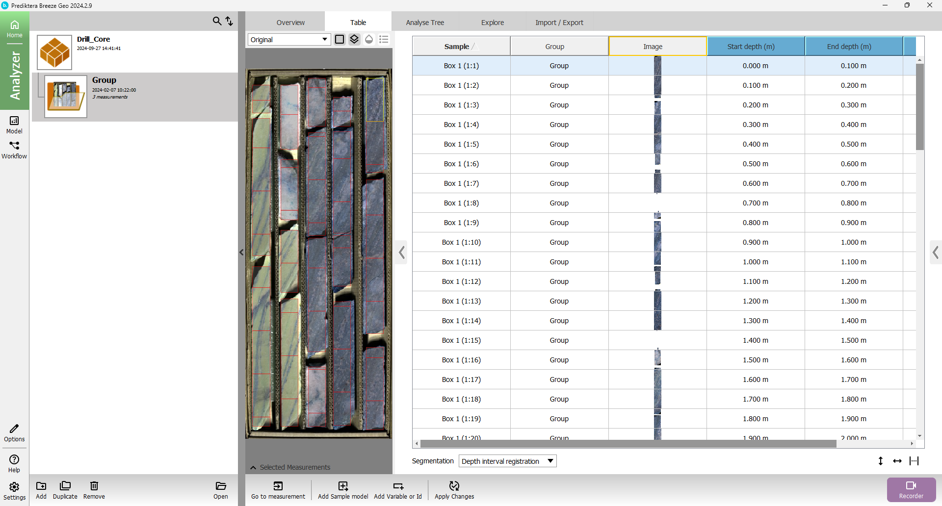
After the changes have been applied there will be three rows in the table one each for the three images. The segmentation uses the core logging from the previous section to segment out the core from the box by defining the area of pixels from the whole image to be processed. Left-click on any of the other rows in the table to see the segment for that image.

Go back to the Analyze tree and press the circle called “Depth registration”.

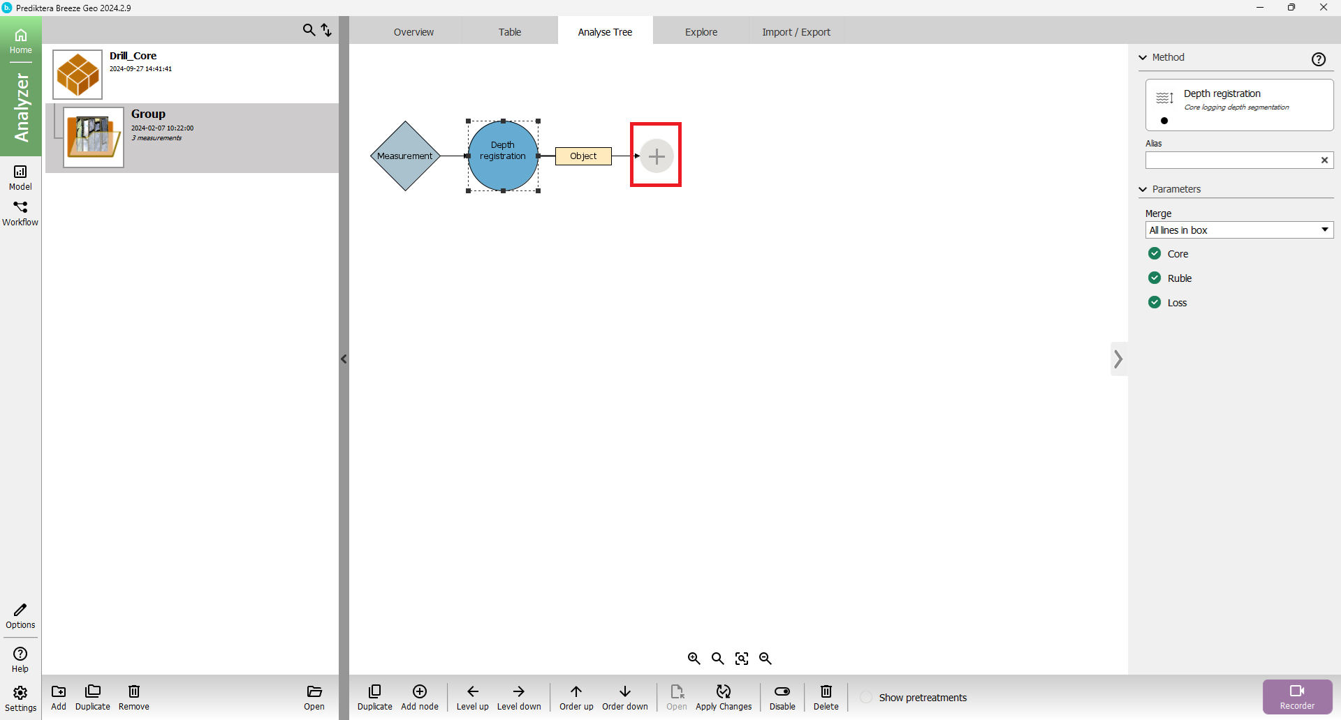
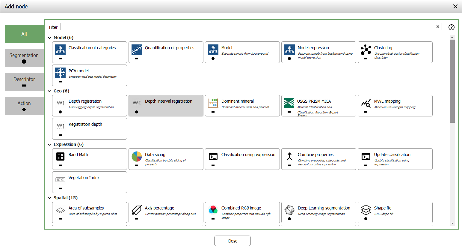
Press the plus sign and add the Depth interval registration

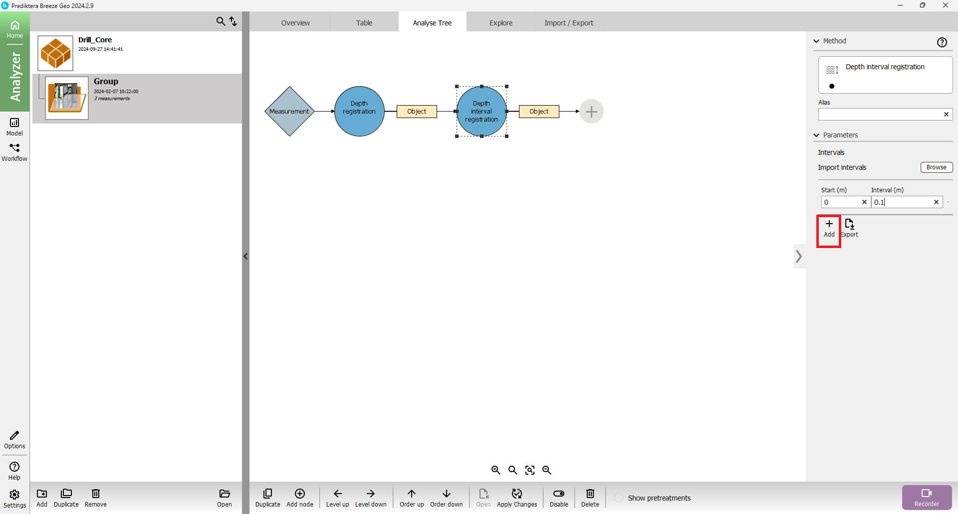
In the menu to the right, the interval length and start depth can be entered. To create 10 cm intervals, enter "0.1" under interval and press "Add”.

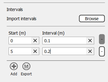
To add a different interval length at a specific depth, press "add". In the new empty row, inter 5 in the start and 0.2 in the interval. Adding this second interval will create 20 cm intervals starting at 5 meters. So, from 0-4.99 meters, 10 cm intervals will be applied, and then at 5 meters, 20 cm intervals will be generated. If you add a second row like here we will have an interval length of 10 centimeters between 0-5 meters and after 5 meters the interval length will be increased to 20 centimeters for the rest of the logged core.

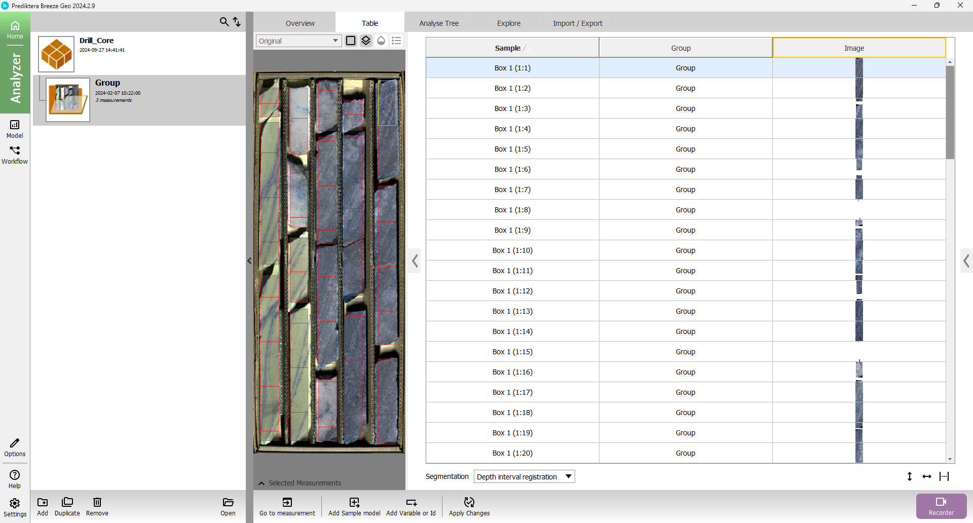
Go back into the table view and press “Apply changes”. To see the changes we need to change the segmentation level which is done below the table change from “Depth registration” to “Depth interval registration”. You will now see that we have more segments in the table.

To add the start, end, and length information of each interval, navigate back to the Analyse Tree in the group level.

Press the circle called “Depth interval registration” and press the plus sign.

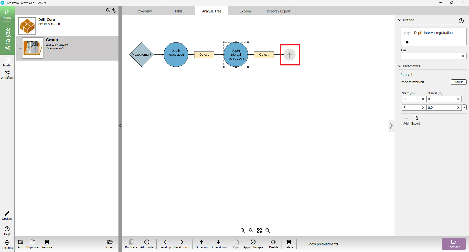
Add the descriptor called Registration depth

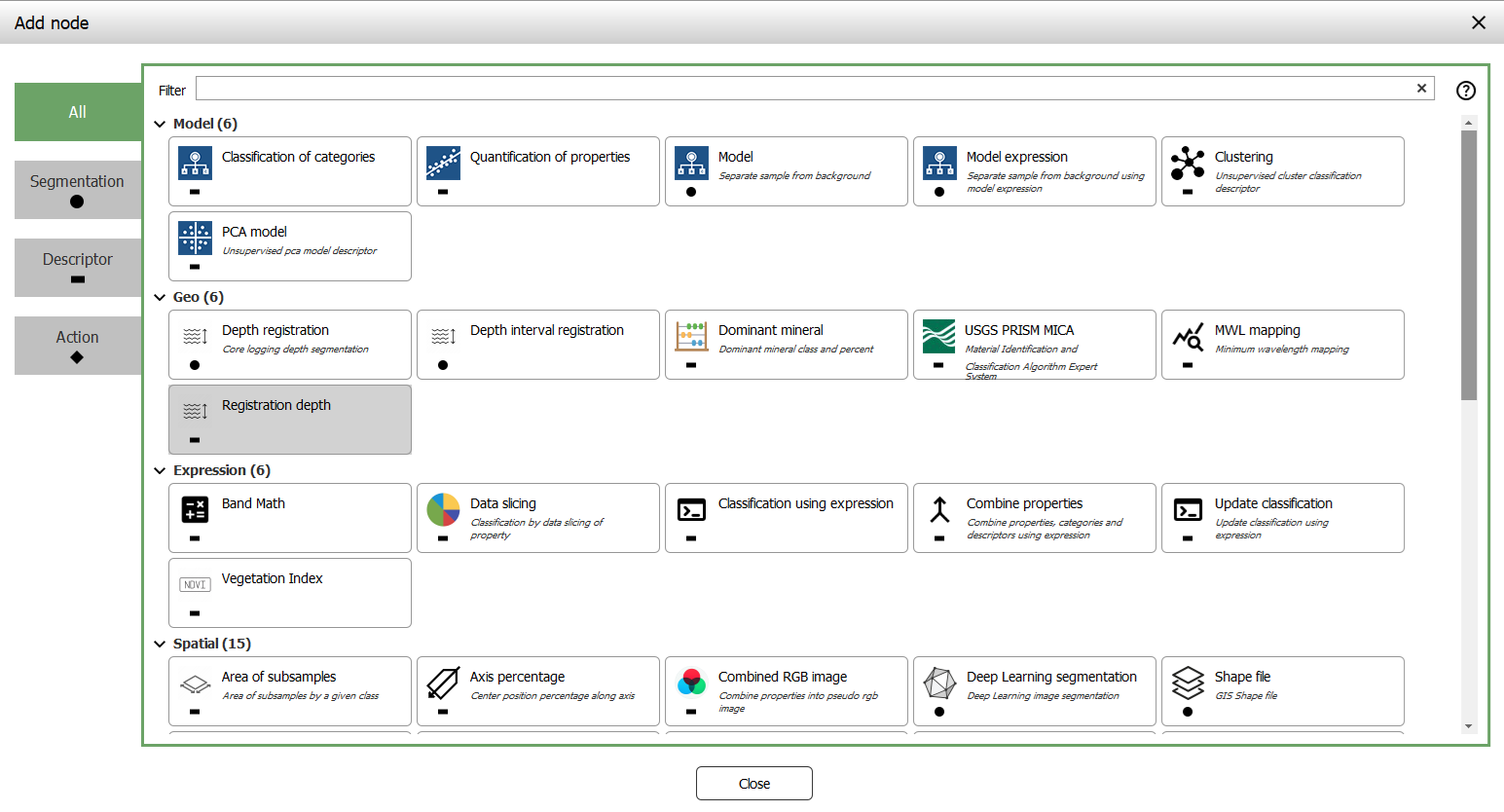
In the Analyse Tree we now have a rectangle with the name “Start depth (m)”. Press it and press the duplicate button two times.

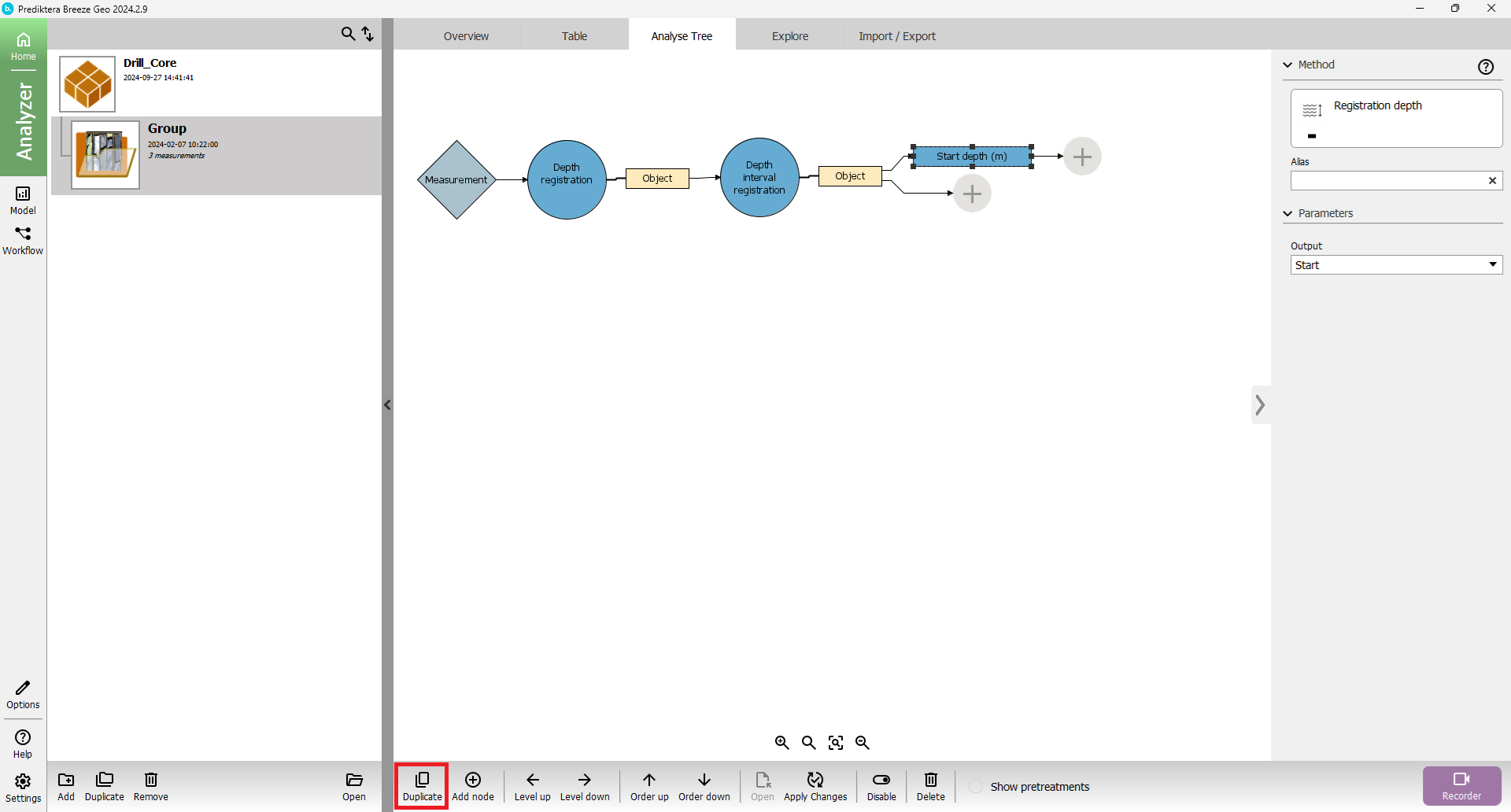
You now have three of the same descriptors. Select the middle descriptor and open the drop down menu to change "Start" to "End"

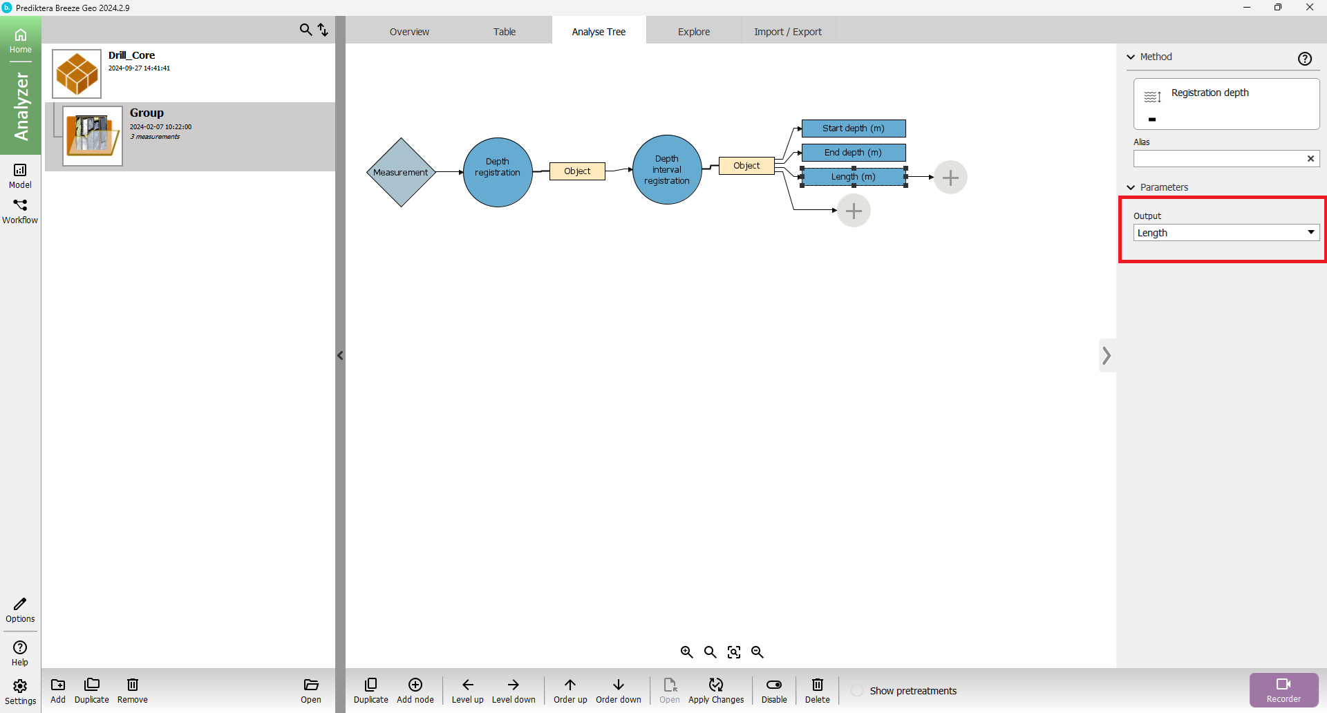
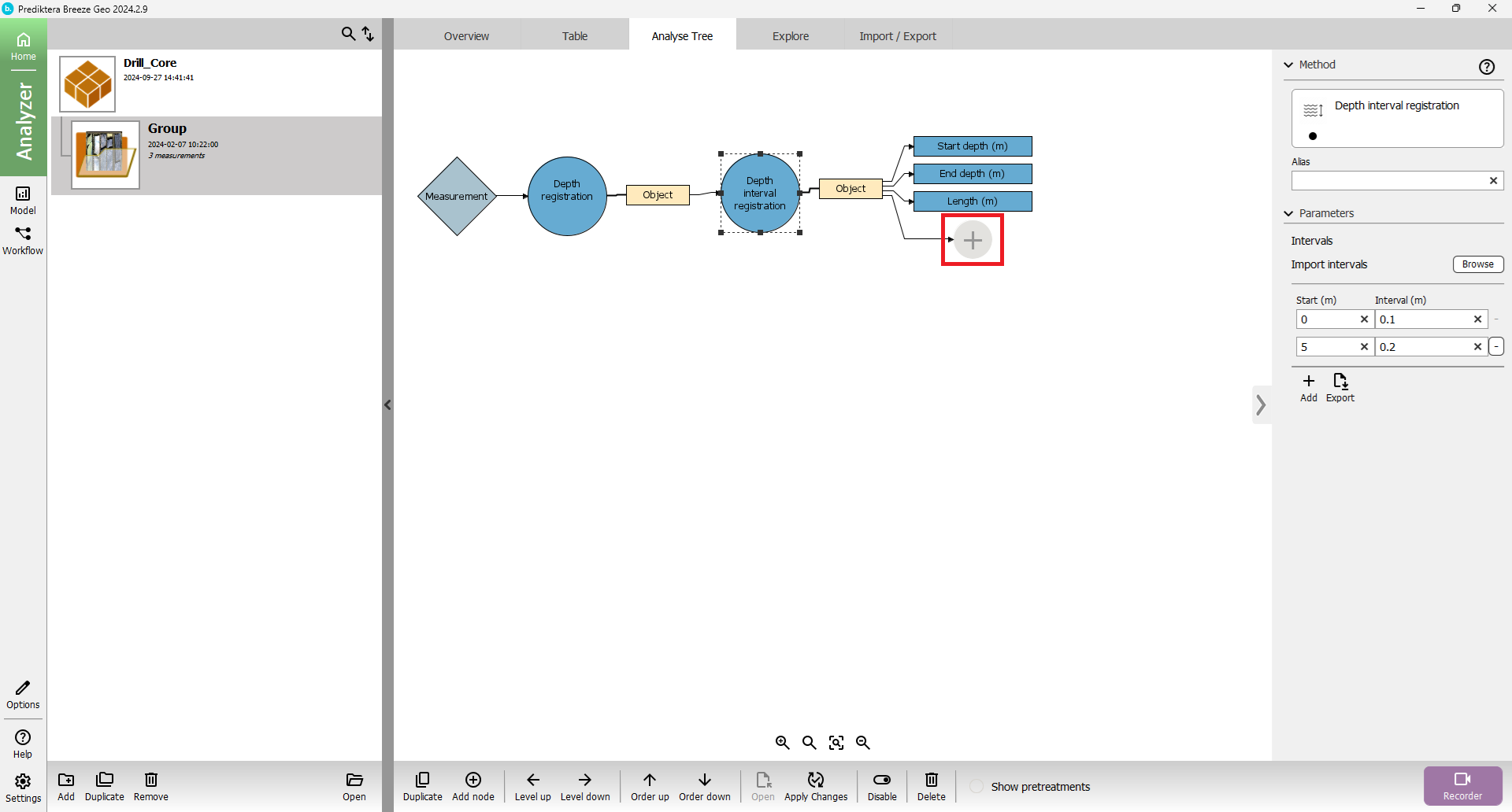
Select the last one and change it to “Length”. The Analyse Tree should now look like the image below.

Go back to the table tab and press “Apply changes”. The table now has three more columns with the start, end, and length information for all of our segments.

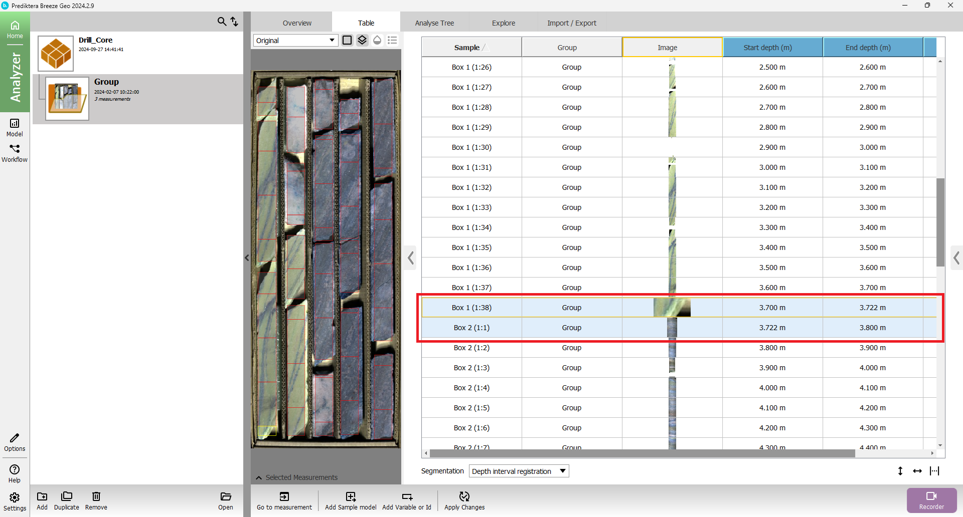
If we scroll down in the table until we get to the end of box 1 and the start of box 2 we can see that we have two segments that are not 10 centimeters. But as you probably already have noticed, the combined length of the segments added comes to 10 centimeters. When exporting the table into a CSV file the analysis of these two segments will be combined as one.

Classification and analysis using USGS

Now when the boxes are segmented and put into intervals we can start adding the analysis tools.

Go to the analyze tree tab and press the “Depth interval registration” and the plus sign.

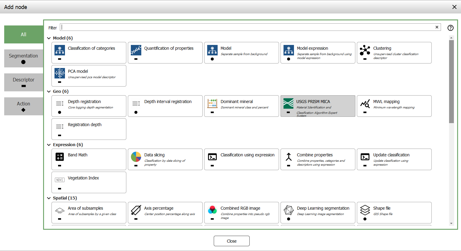
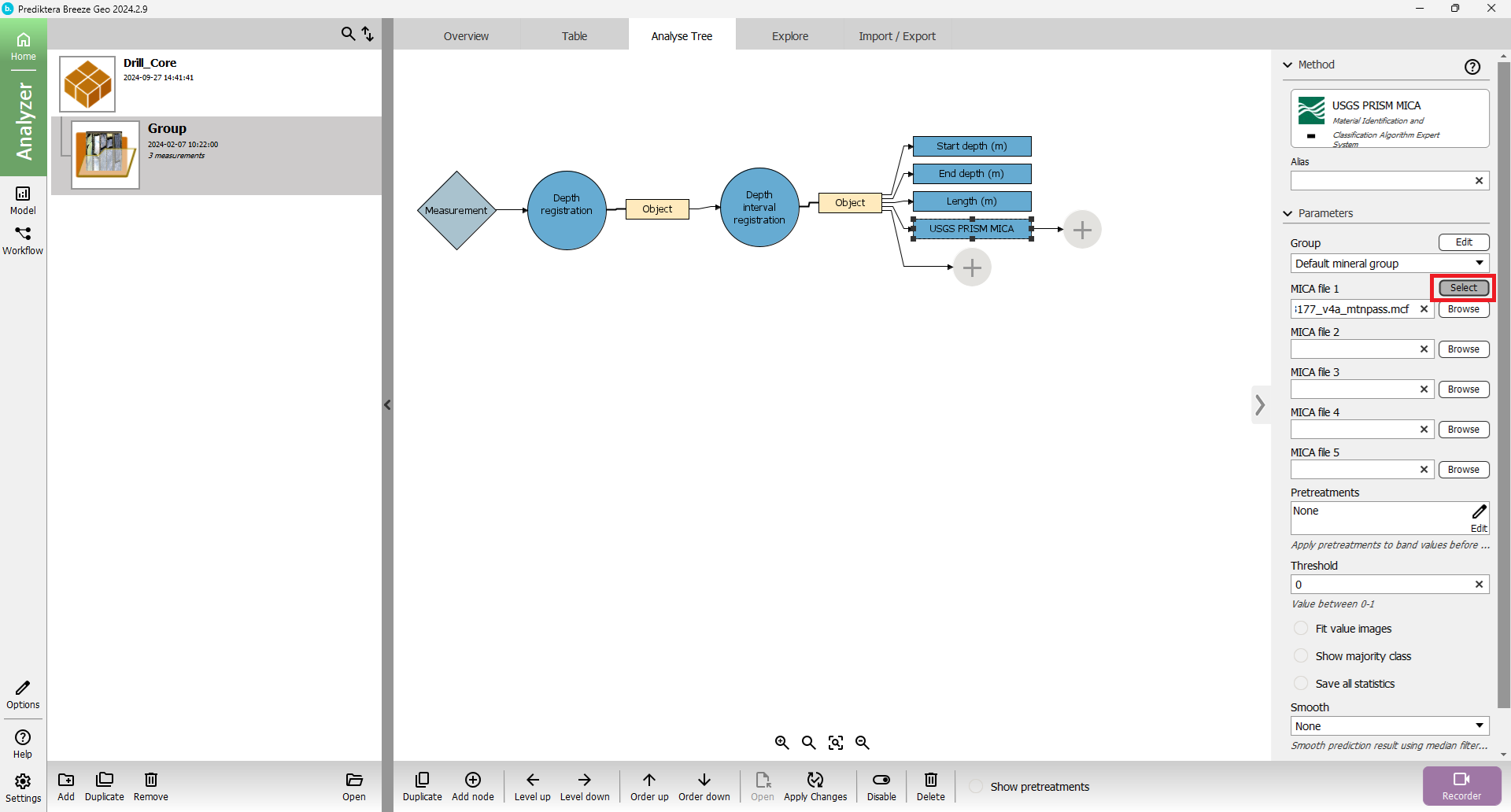
Select the descriptor called Mica expert system

In the menu to the right press the select button.

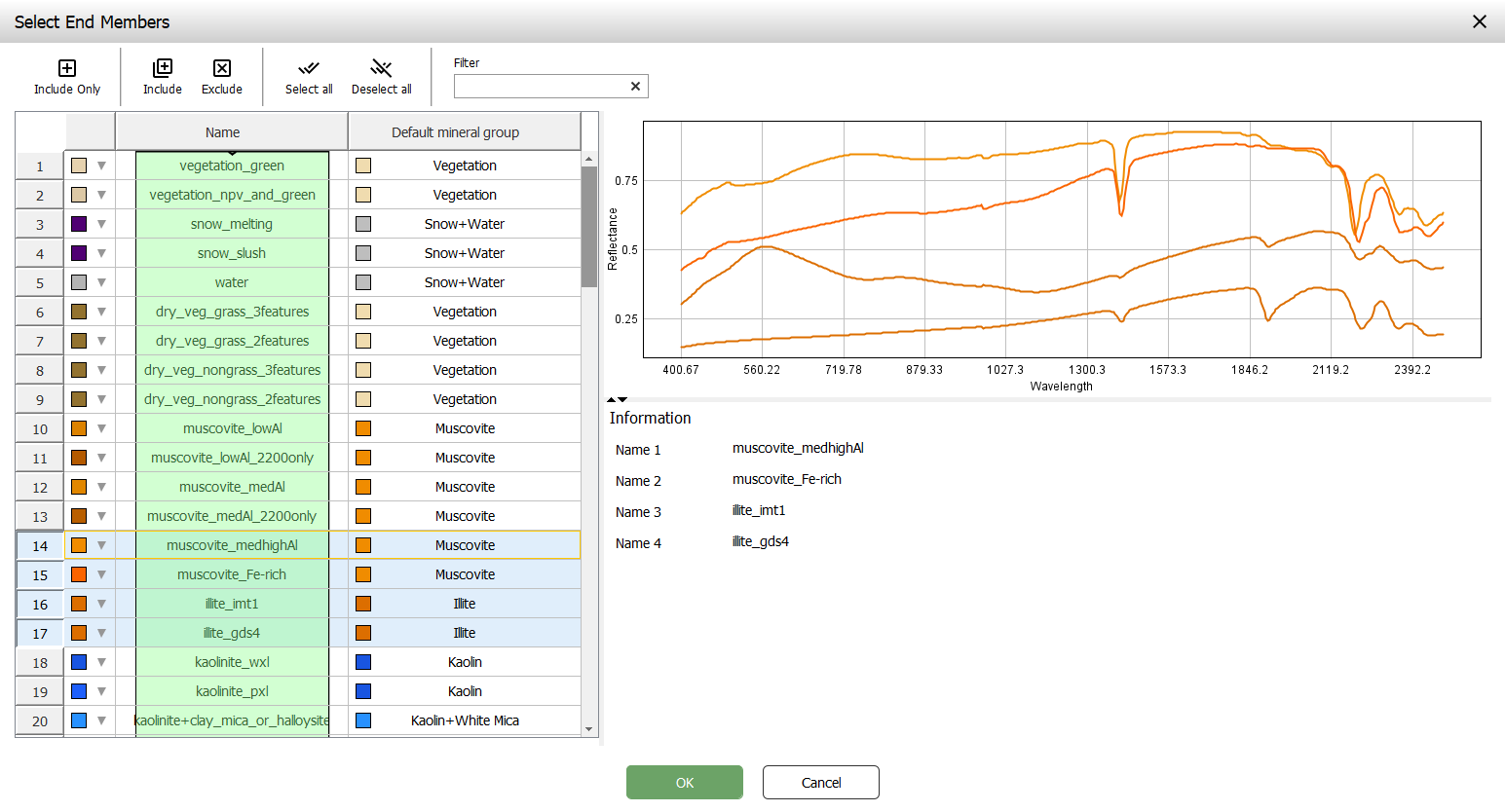
We can now see all the spectrum that is used by the Mica expert system for its classification.

You can select some end members and see the spectrum when you are done exploring the spectrum press “OK”.

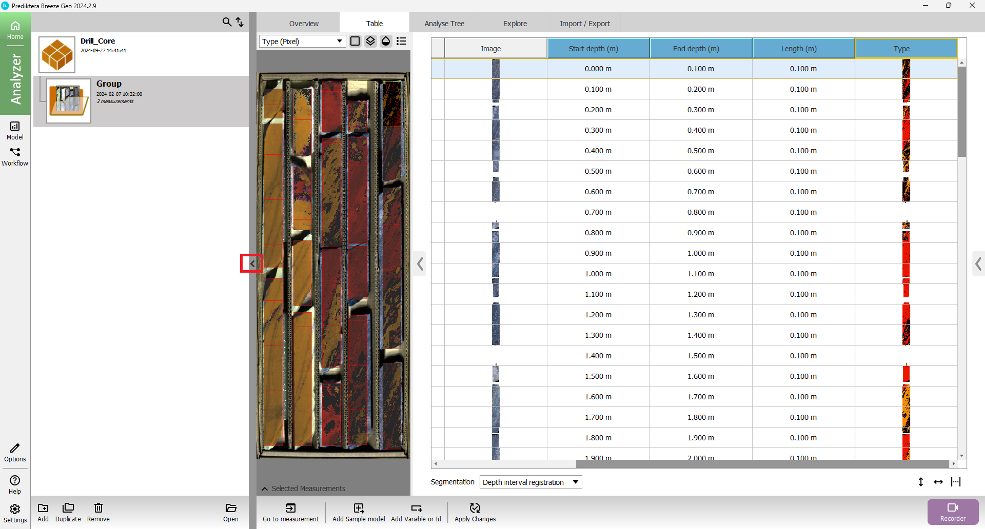
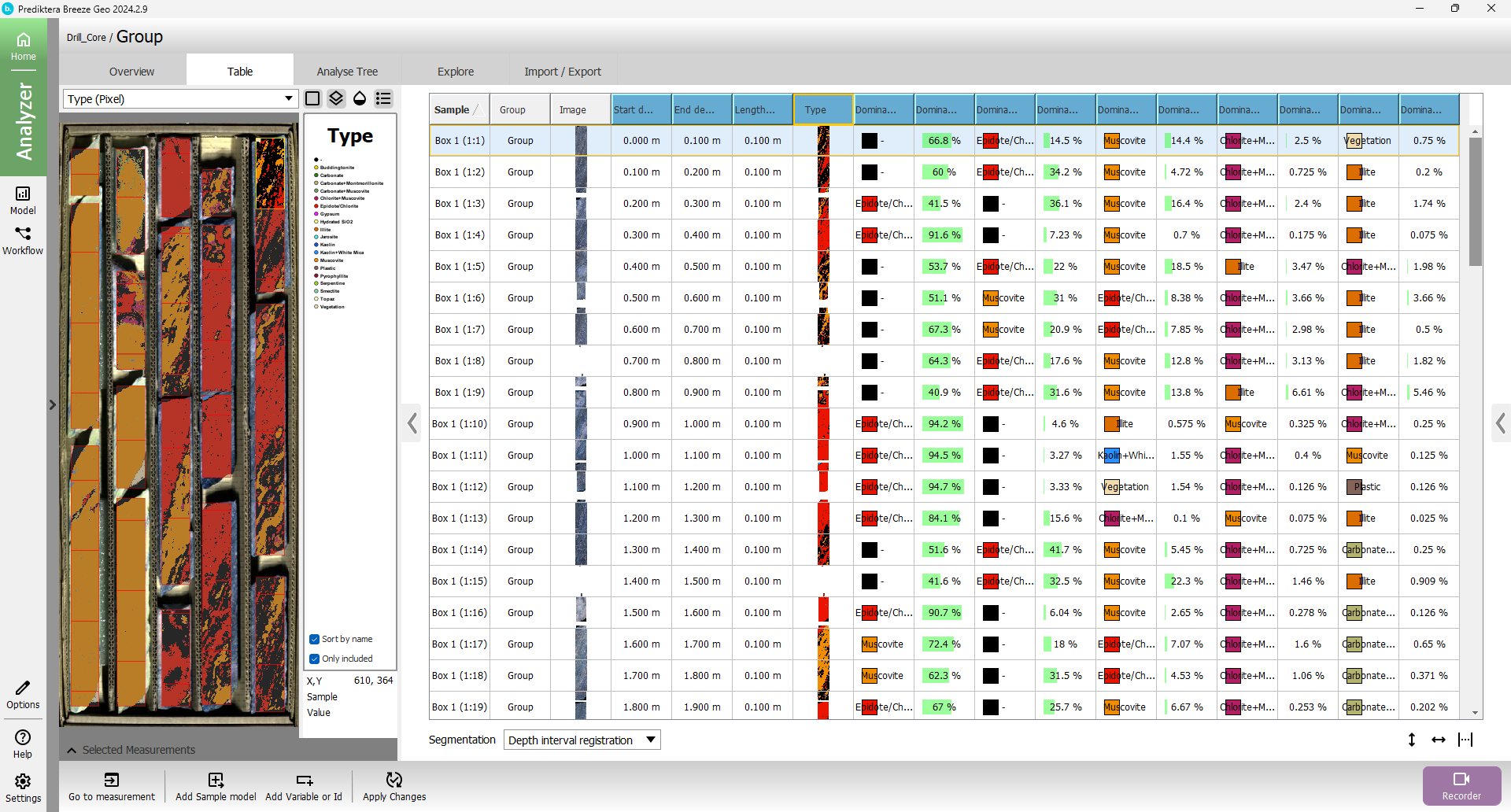
Go to the table view and press “Apply changes”. Now a new column with the output from MICA expert system will appear in the table. Press the column and the pseudo RGB image will change for the classification output.

Press the chevron to minimize the left menu with the groups.

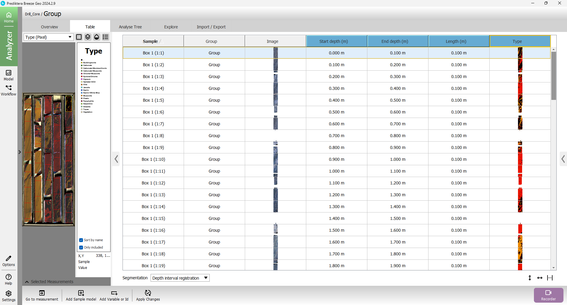
Press to see the legend of the classification.

To get the legend larger fist hover the mouse over the right gray border until the mouse changes to

and drag it to the right.

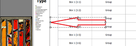
This will add more room for the image. Now hover the mouse over the left gray border of the legend and drag it to the left.

The legend should now be larger and more easy to read.

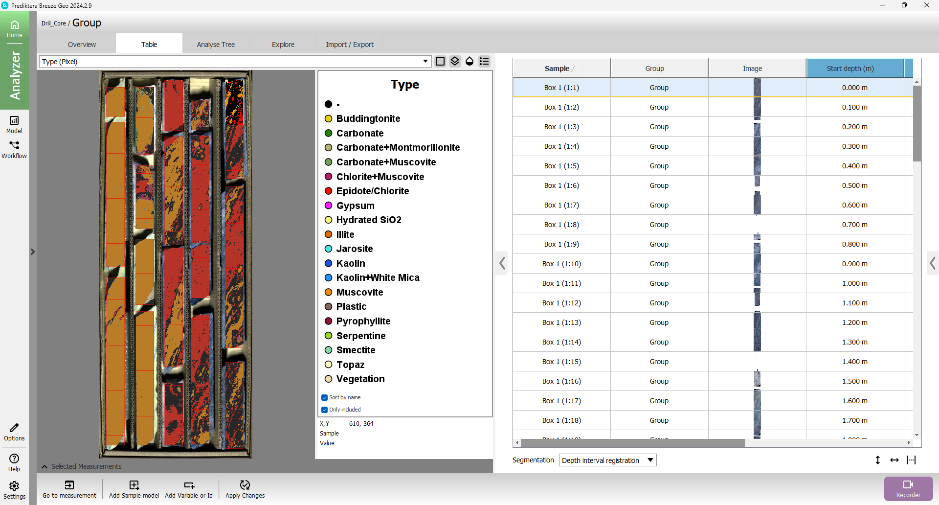
If you hover your mouse over the image you can also see the classification of that pixel below the legend.

Feel free to scroll down in the table to see the results on Box 2 and Box 3.

We will now go back to the Analyze Tree press the rectangle for the Mica expert system and press the plus sign behind it.

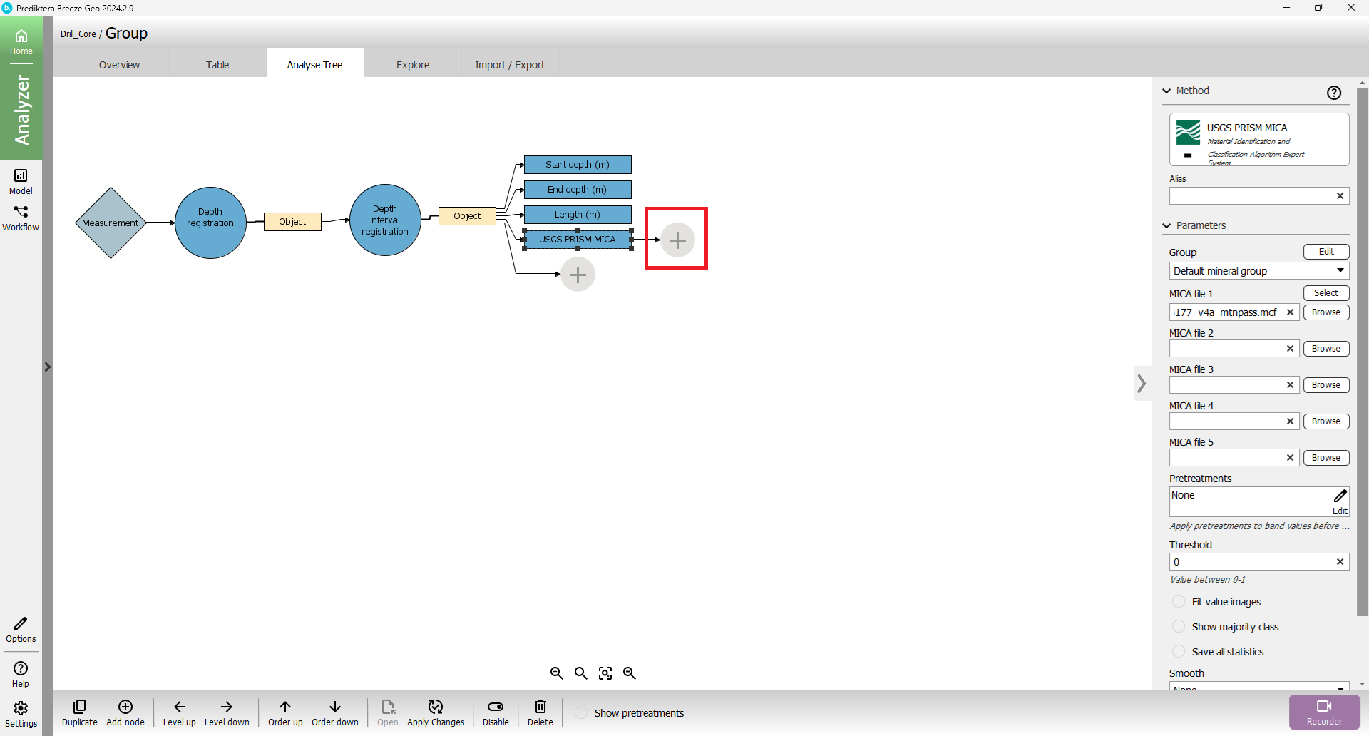
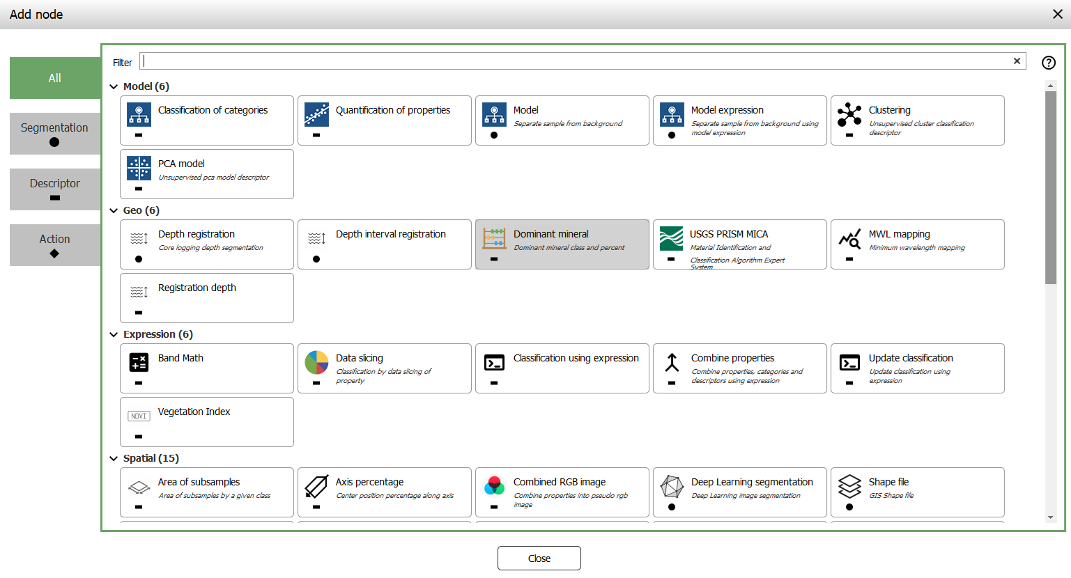
Add the descriptor Dominant mineral.

Change the number from 10 to 5.

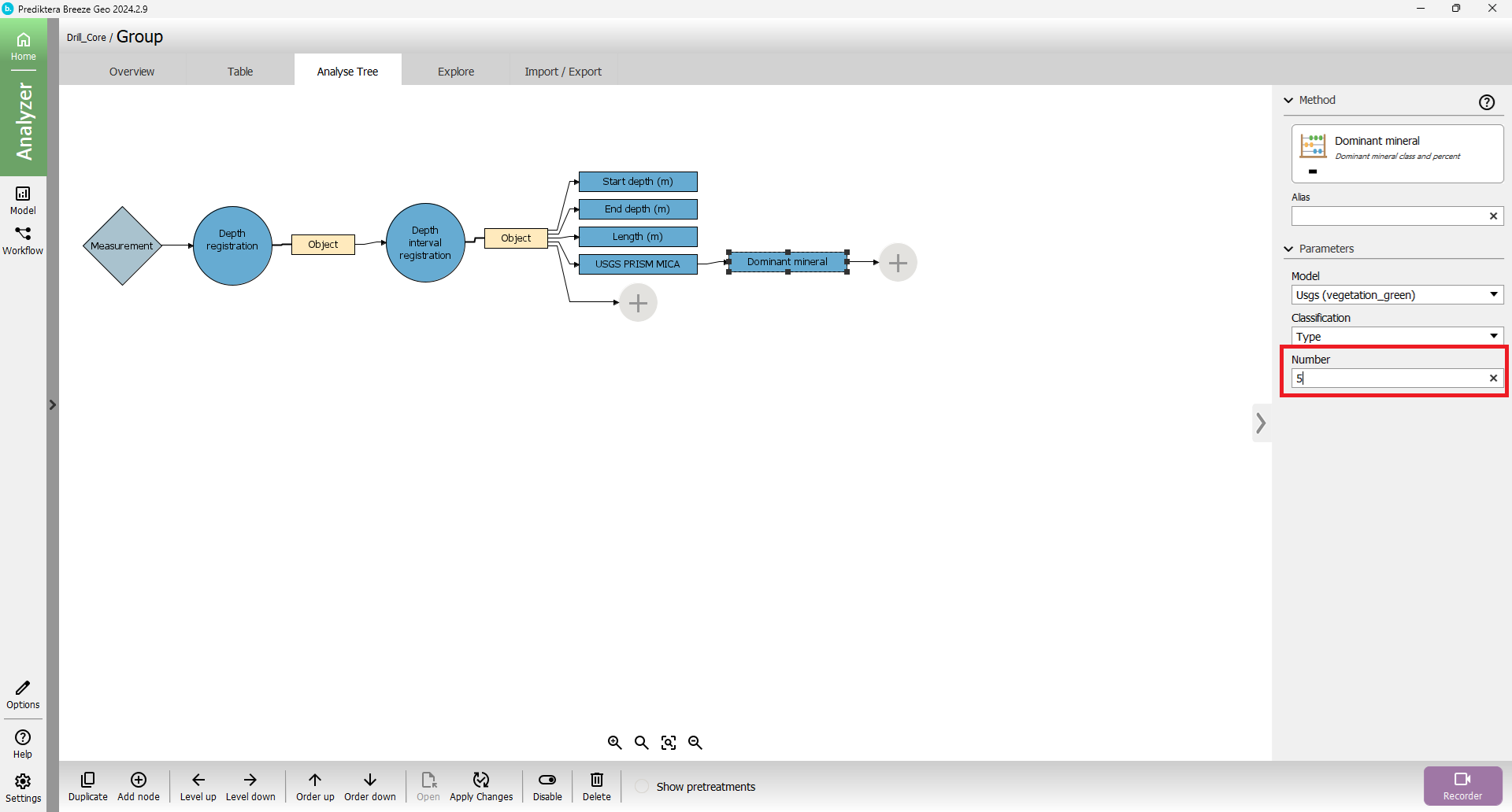
Go back to the table view and press “Apply changes”. In the table five new columns will appear, they contain information about the five most common mineral classifications based on the Mica expert system. The abundance of the minerals is calculated using a pixel count.

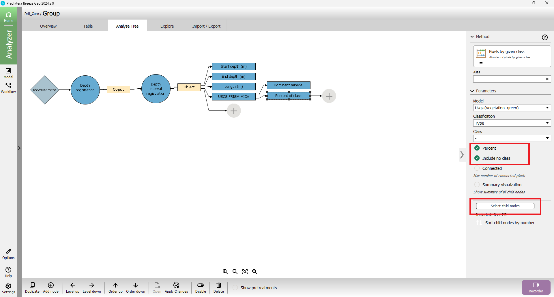
Instead of showing the most dominant mineral you can also select the descriptor Pixel by given class.

Go to the Analyse Tree and add the descriptor after the Mica expert system. Scroll down in the node selection window until you find the Pixel by the given class descriptor. After you have added the descriptor your analyze tree should look like this.

In the menu to the right check “Percent” and “Include no class”. After you can check the two options press the “Select child nodes” to decide which minerals you want to calculate the pixel percentage for.

Press “Epidote/Chlorite” and press Include

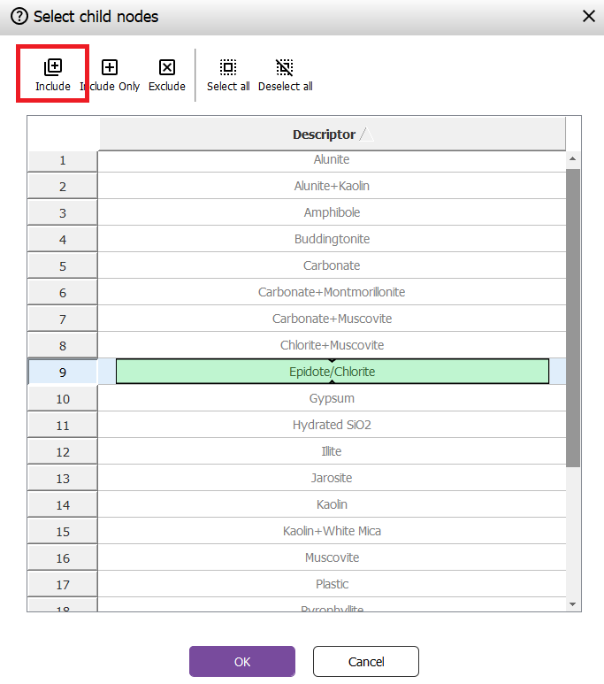
Do the same for Muscovite and then press OK.

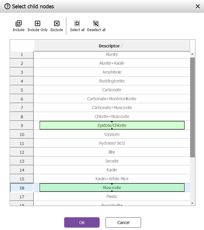
Go to the table view and press “Apply changes”. Two new columns have been created and you can now follow the mineral content of either Epidote/Chlorite or Muscovite throughout the depth of the drill hole.

Export result into CSV

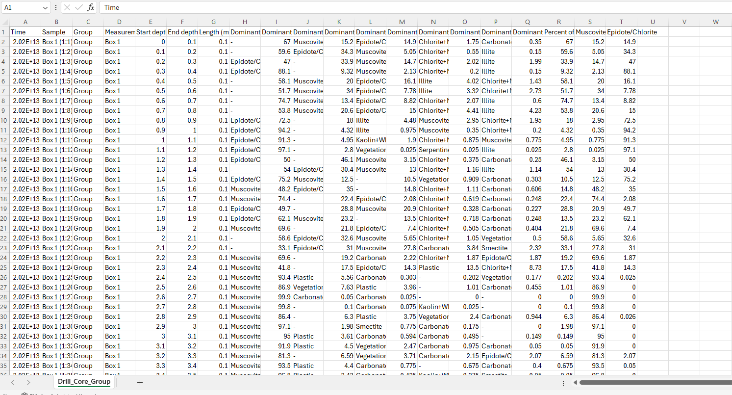
When you are done with the analysis you can export the result from the table into a CSV which can be shared with people that do not have access to the software.

Go to the Export tab select Export to CSV and press “Apply”.

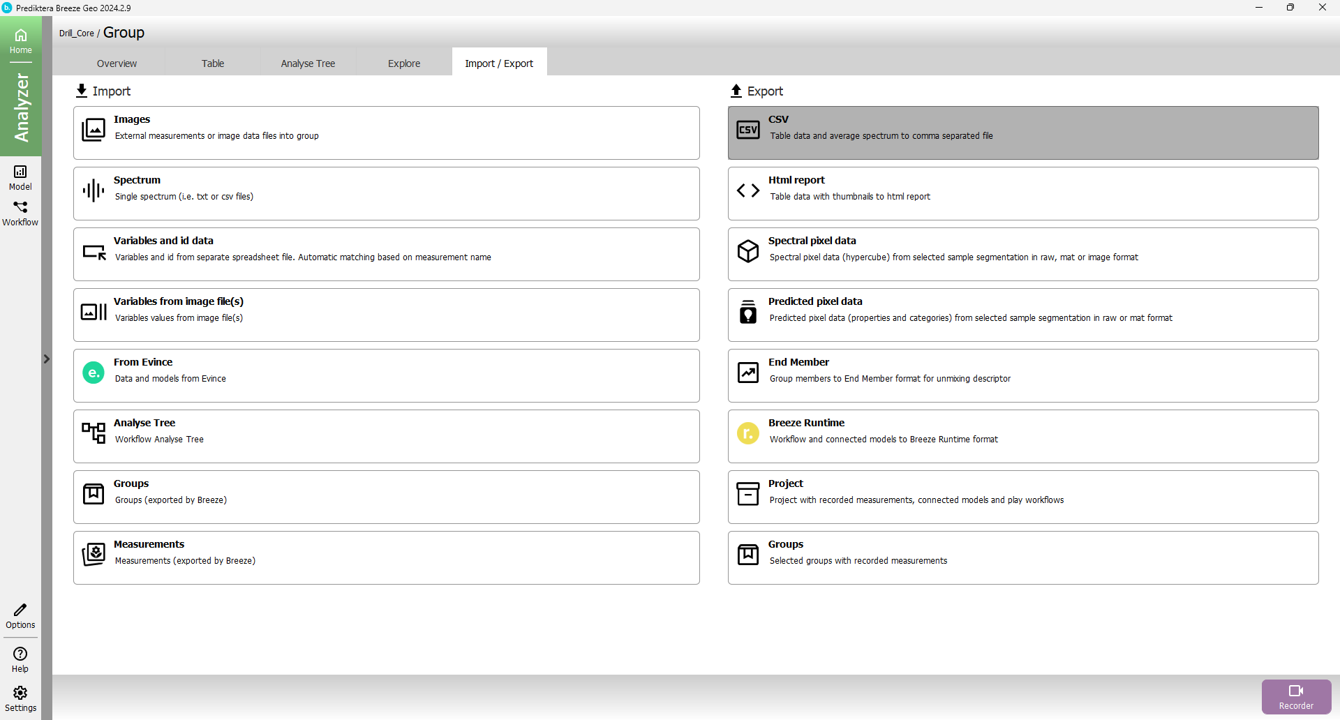
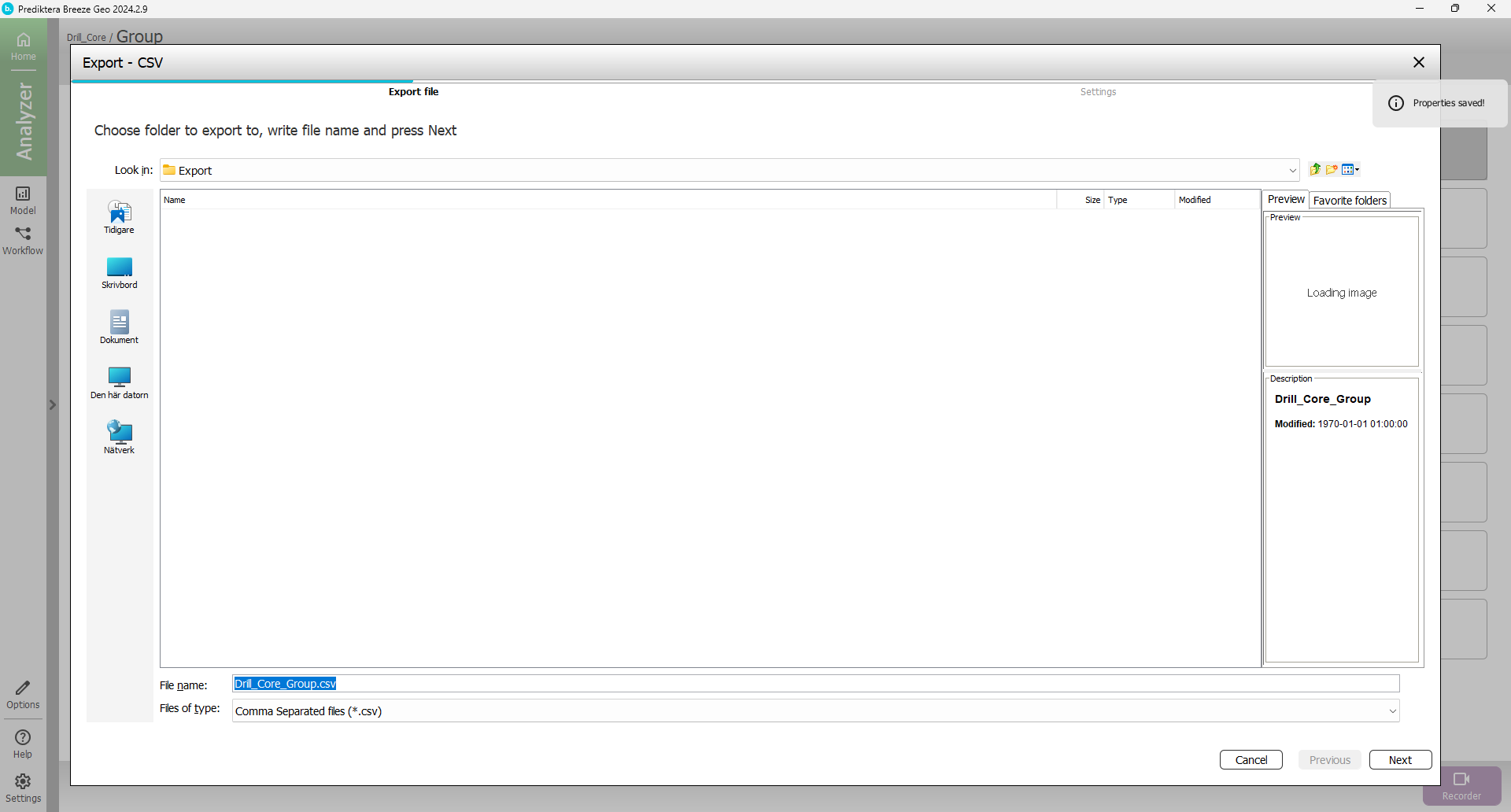
You can now select where you want to store the CSV. The default location is in a folder within the Breeze workspace structure. when you have selected a location press “Next”.

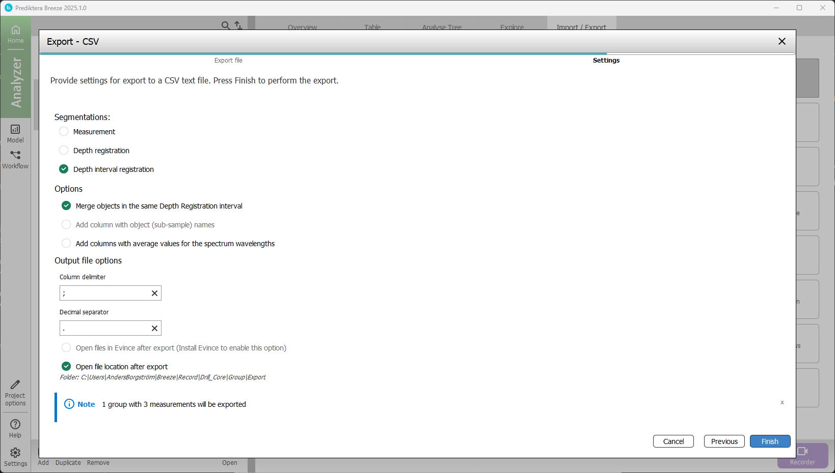
Uncheck the “Include average spectrum wavelength value” we do not need to add an average spectrum for each segment into the CSV,but leave the box for “Depth interval: merge samples with same index” this will combine the segments between boxes which we discussed after adding the depth interval segmentation.

Press “Finish”

A CSV file is now created containing all the information from the table in Breeze