Segmentation guide

This guide will show you how to use the different types of image segmentation that are available in Breeze. To see the list of available segmentation look at the document Segmentations .

The method “Segmentation by model” is covered in the tutorials Quantification of powder samples and Classification of nuts step 1, and that will not be covered in this guide.

General instructions

Analyse Tree

The other view is to open the “Analyse Tree” tab. Here you have a graphical presentation of the different steps in your segmentation. By clicking on a node in your “tree”, you can change the settings for it in the menu on the right. Under the picture of the tree you there is a menu to Add, move or remove nodes. The options in the “Analyse Tree” view are the same as under Project Settings.

Switching between different Segmentations

You can change the segmentation that you want to look at by using the menu under the table.

Examples

Intensity segmentation

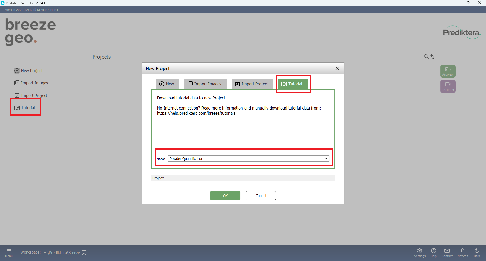
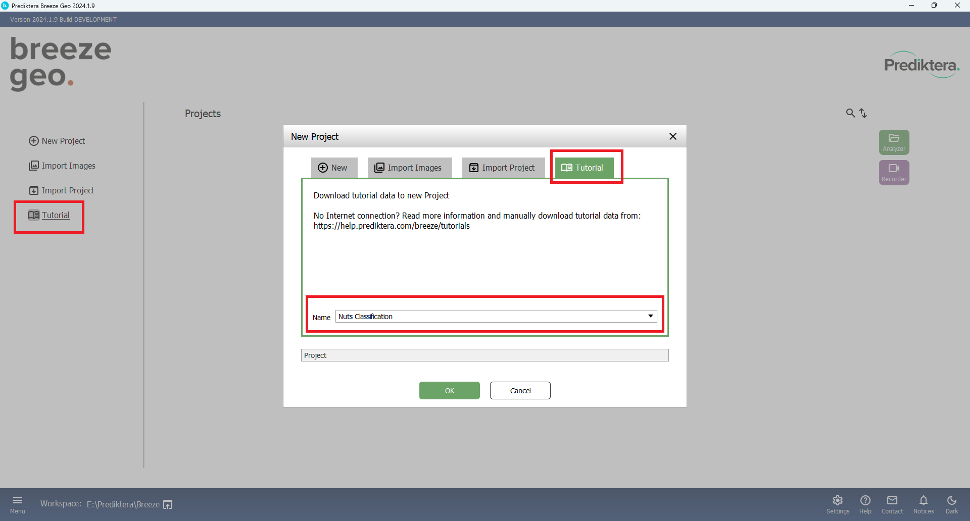
Create a new Project “Tutorial. Choose Tutorial and “Powder Quantification”.
Press OK

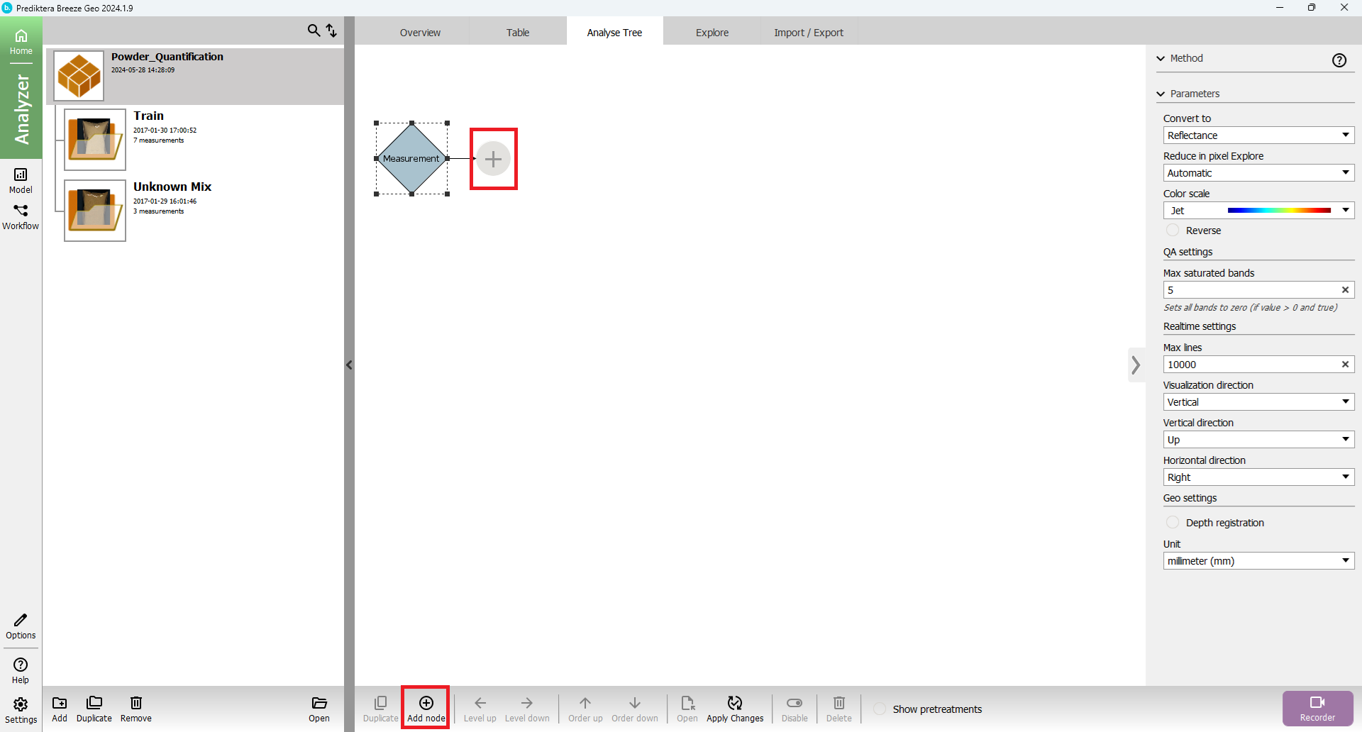
Press “Analyzer” button and the view should look like this:

Press “Analys Tree” tab and add a new node of segmentation type “Intensity by clicking the measurement node in the tree and “Add new node” (or the plus node)

Search for “Intensity” in the Filter text field och browse in the Segmentation tab for the Intensity node type:

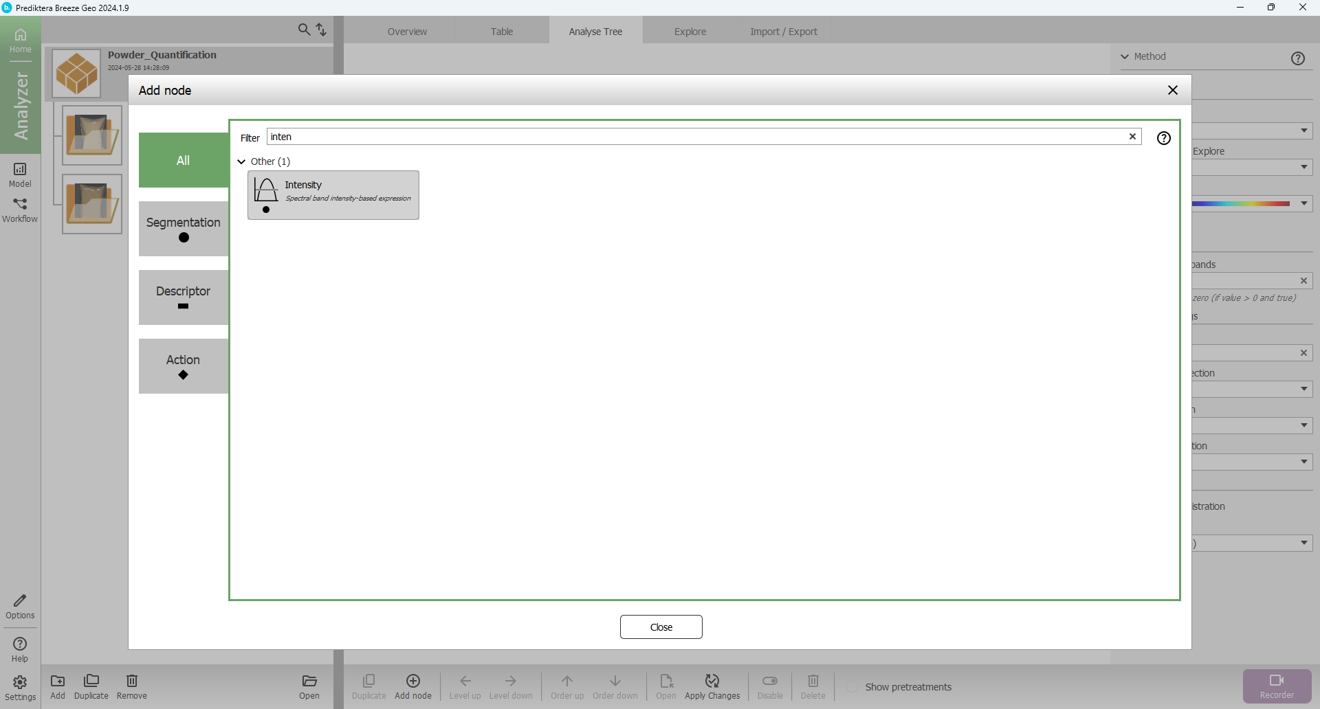
Segmentation by Intensity uses a logical expression to segment the sample objects. The logical expression can compare different spectral bands with each other or by a set value of intensity. The spectral band variable format is b[band index] and starts with a b followed by the band index; for example, b10 mean band index 10.

See Intensity for more information

The value from the band index is either pseudo absorbance value if data includes white and dark references if-else raw spectral value.

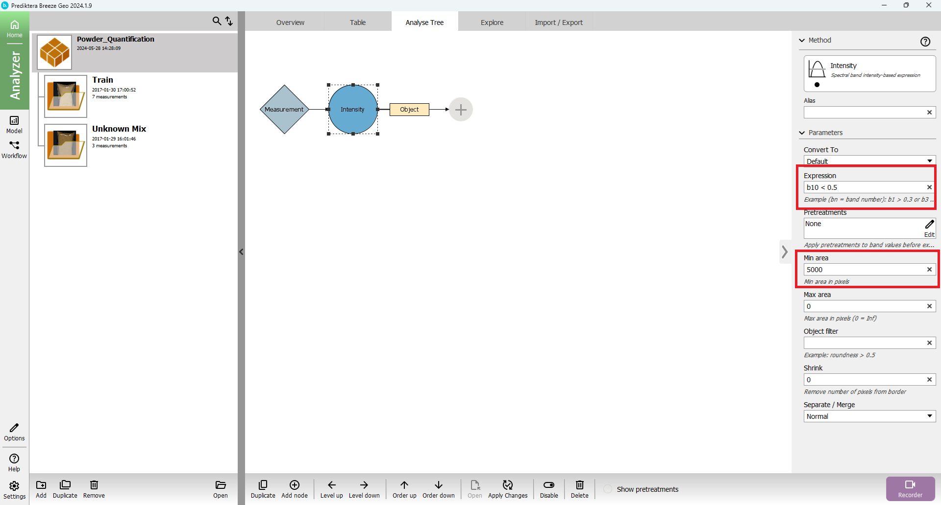
Change “Min area” size to 5000 to exclude small objects

Set “Expression” to b10 < 0.5. This means that band index 10 should be strictly below the intensity of 0.5.

Press “Apply Changes”

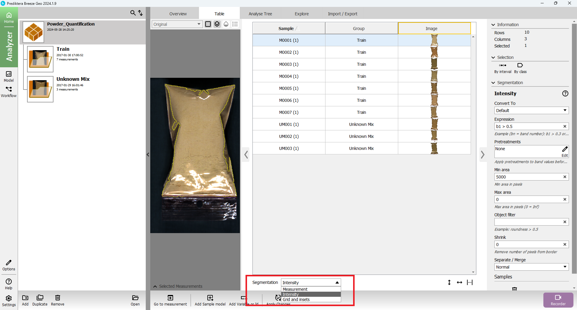
The table view should look like this:

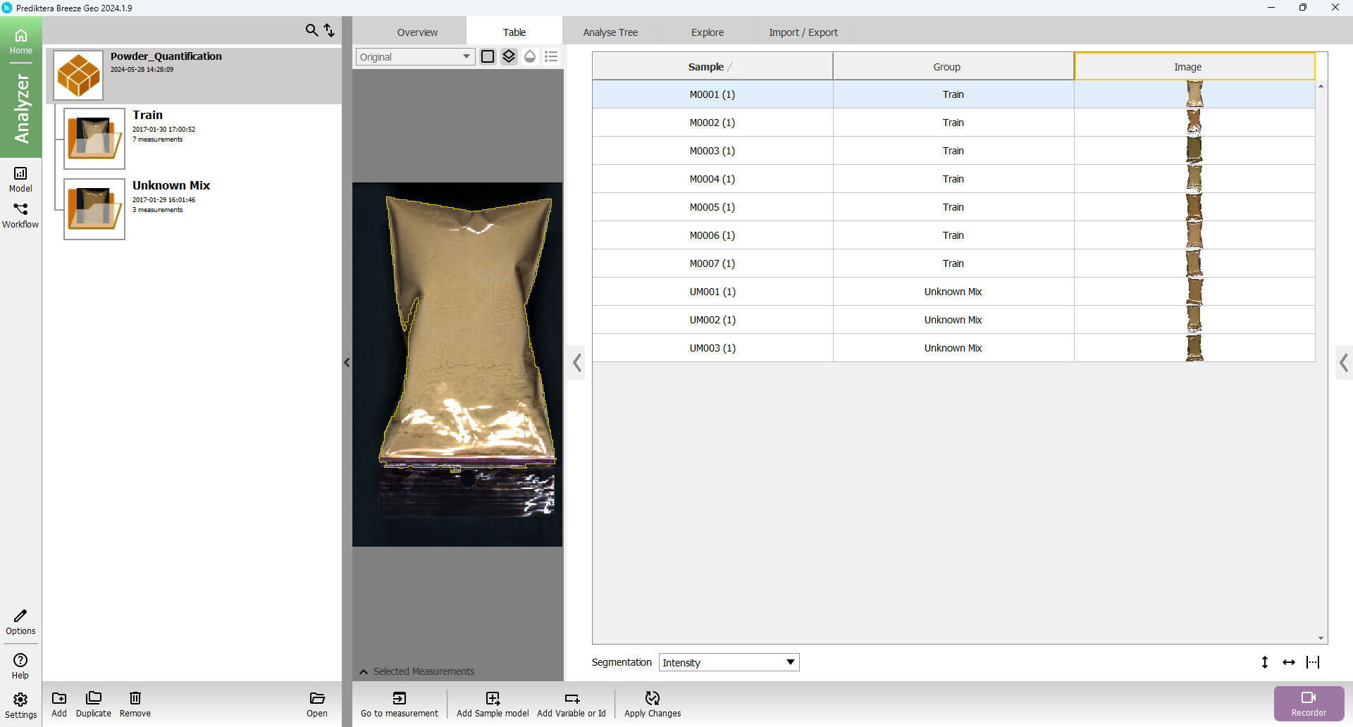
The yellow segmentation selection line is now around the plastic bag in the measurement preview.

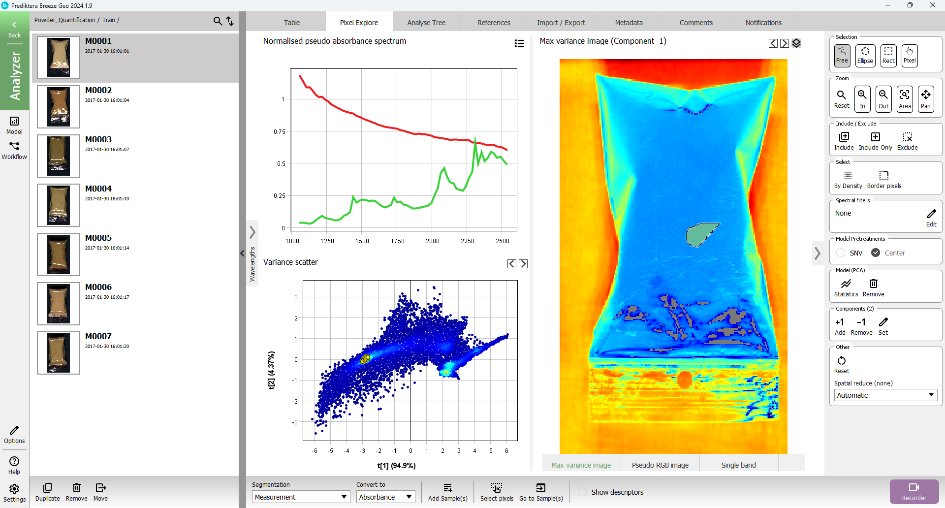
By looking at the “Pixel Explore” tab and selecting a region inside the sample and a region from the background, you can compare the average spectral profiles for the different materials. You can then get an idea of the spectral bands where you have a big difference, and also what intensity value to set.

Grid and Insets segmentation

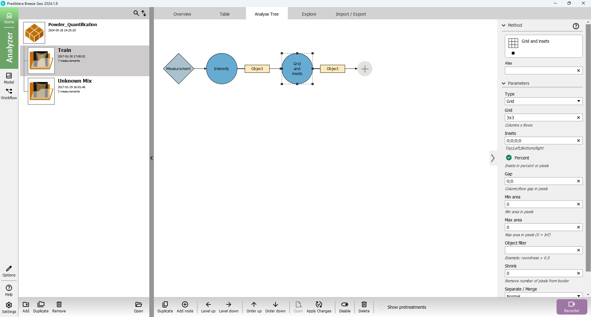
Select the “Intensity” segmentation node in the Analyse Tree and klick Add node (or the plus symbol) and add filter out the “Grid and insets” node.

Change “Insets” to 30 (same as specifying 30;30;30;30 - Top;Left;Bottom;Right)

Change “Percent” to “true” (If the percent is false it will use insets as pixels)

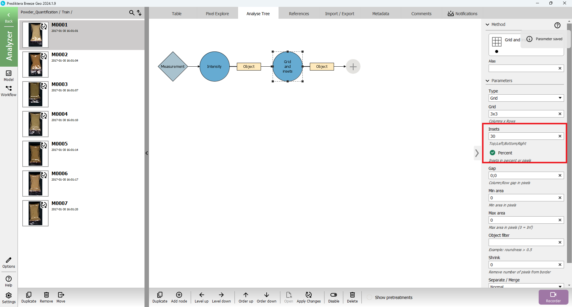
Press “Apply Changes” and then press “Up” button

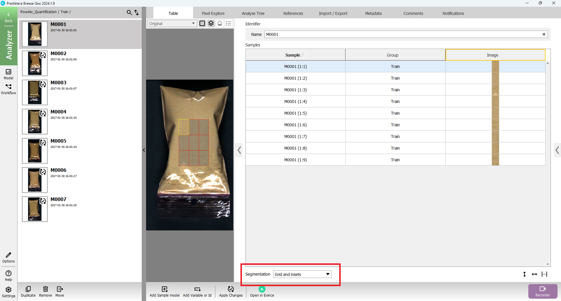
Change “Segmentation” to “Grid and insets” in the drop-down menu.
The view should then look like this.

An inset of 30% has been applied from each side. The sample has then been divided into a 3x3 grid creating 9 sub-sub-samples.

Manual segmentation

Create a new Prject (Press “Tutorial”). Choose Tutorial and “Nut Classification”.
Press OK

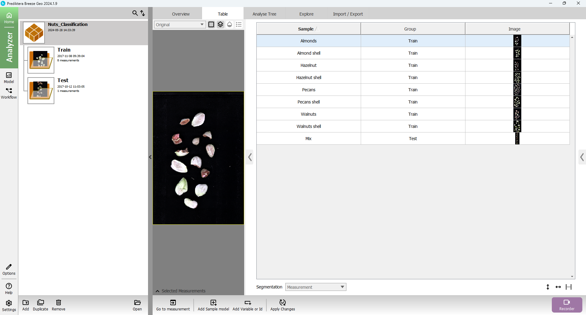
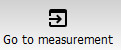
Press “Analyzer” and the view should look like this:

Press “Go to measurement” button on the toolbar

Press “Pixel Explore” tab, click on Model (PCA) “Create” button

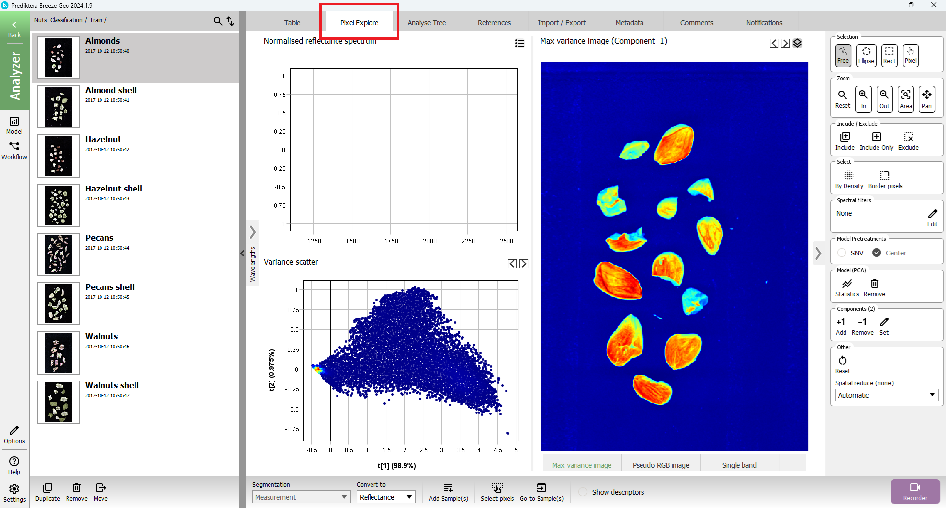
Select area of interest in either “Variance scatter” or “Max variance image”

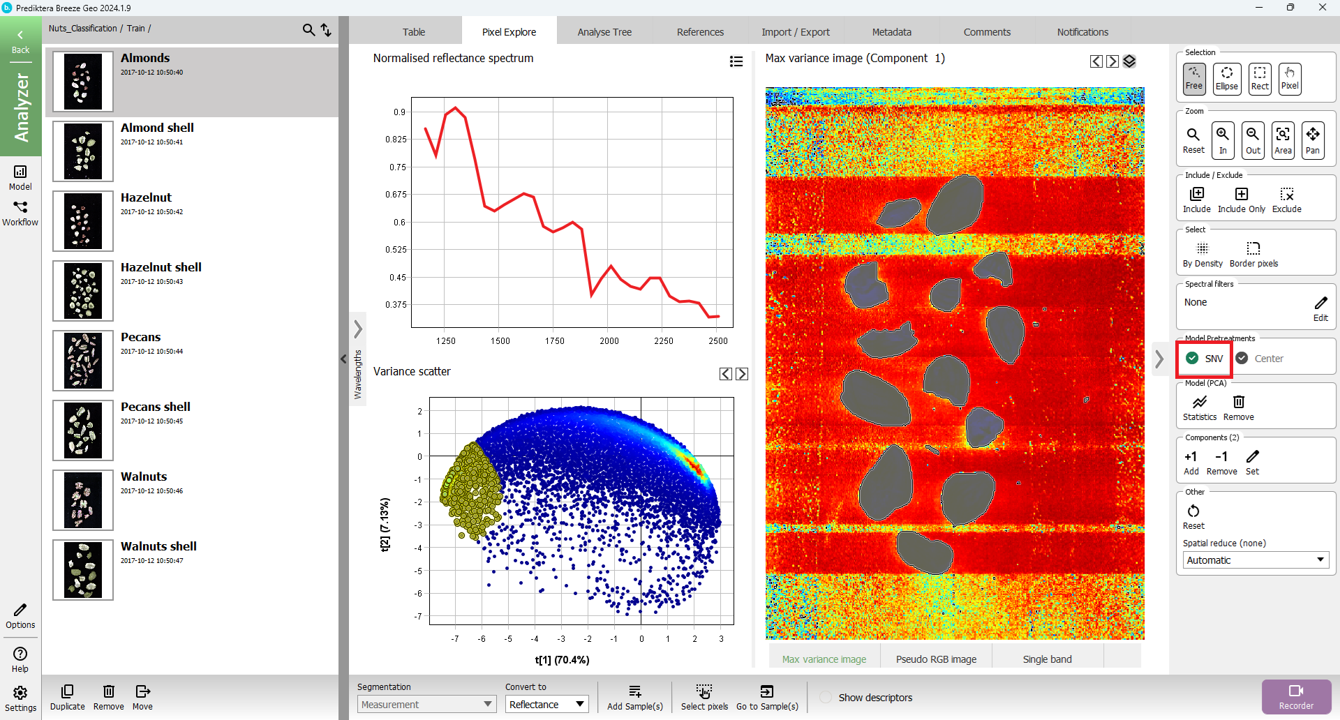
Press “Add Sample(s) from selection” button.

Keep the default options.

Samples are created from the selection and you are back in the “Table” tab

Adjust segmentation settings by toggling the right settings panel

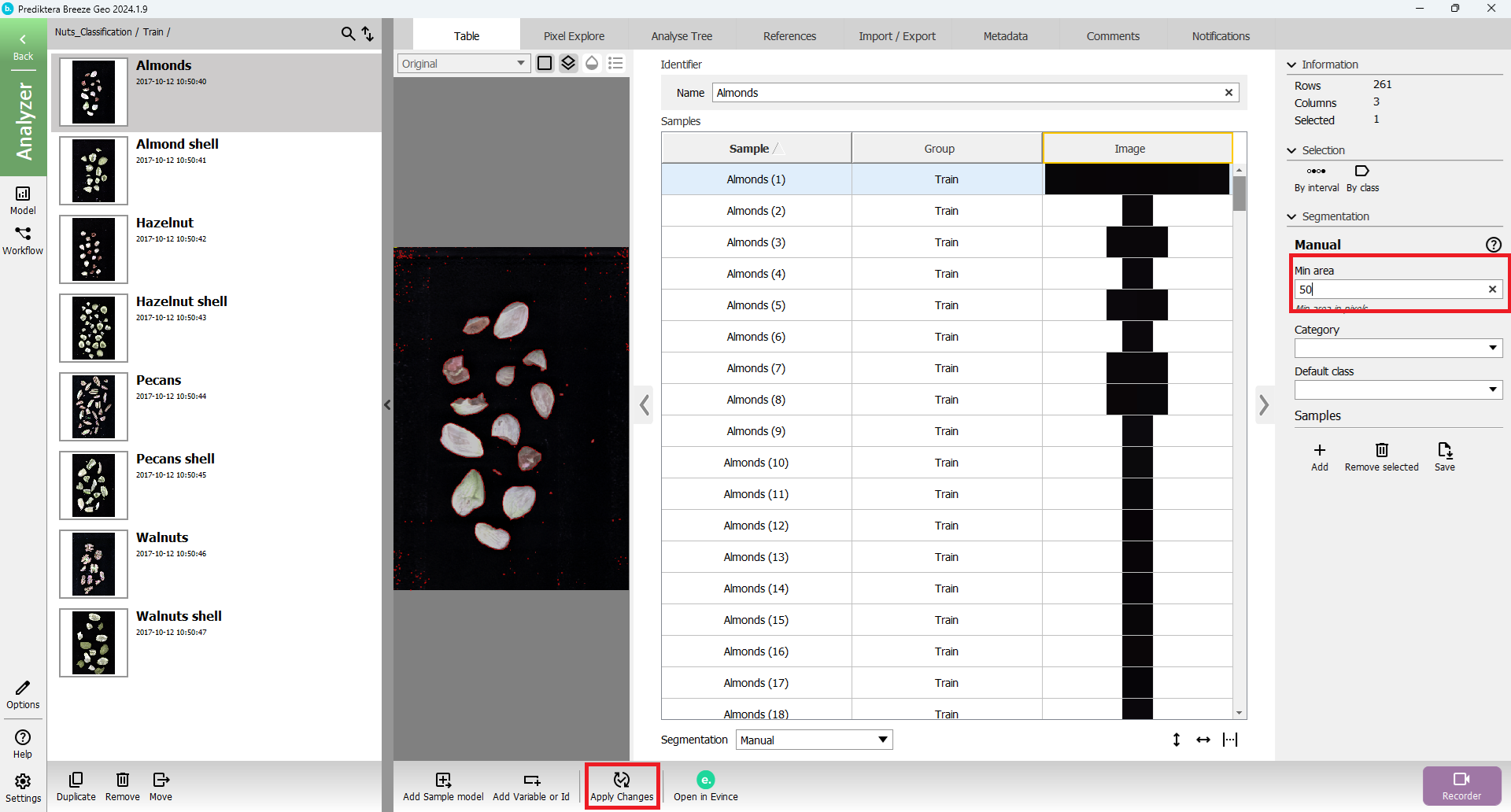
Change for example the “Min area” to 50 and then press “Apply Changes”

The unwanted object can be removed by pressing the “Remove selected Samples(s)” button in the settings panel.

Representative spectrum

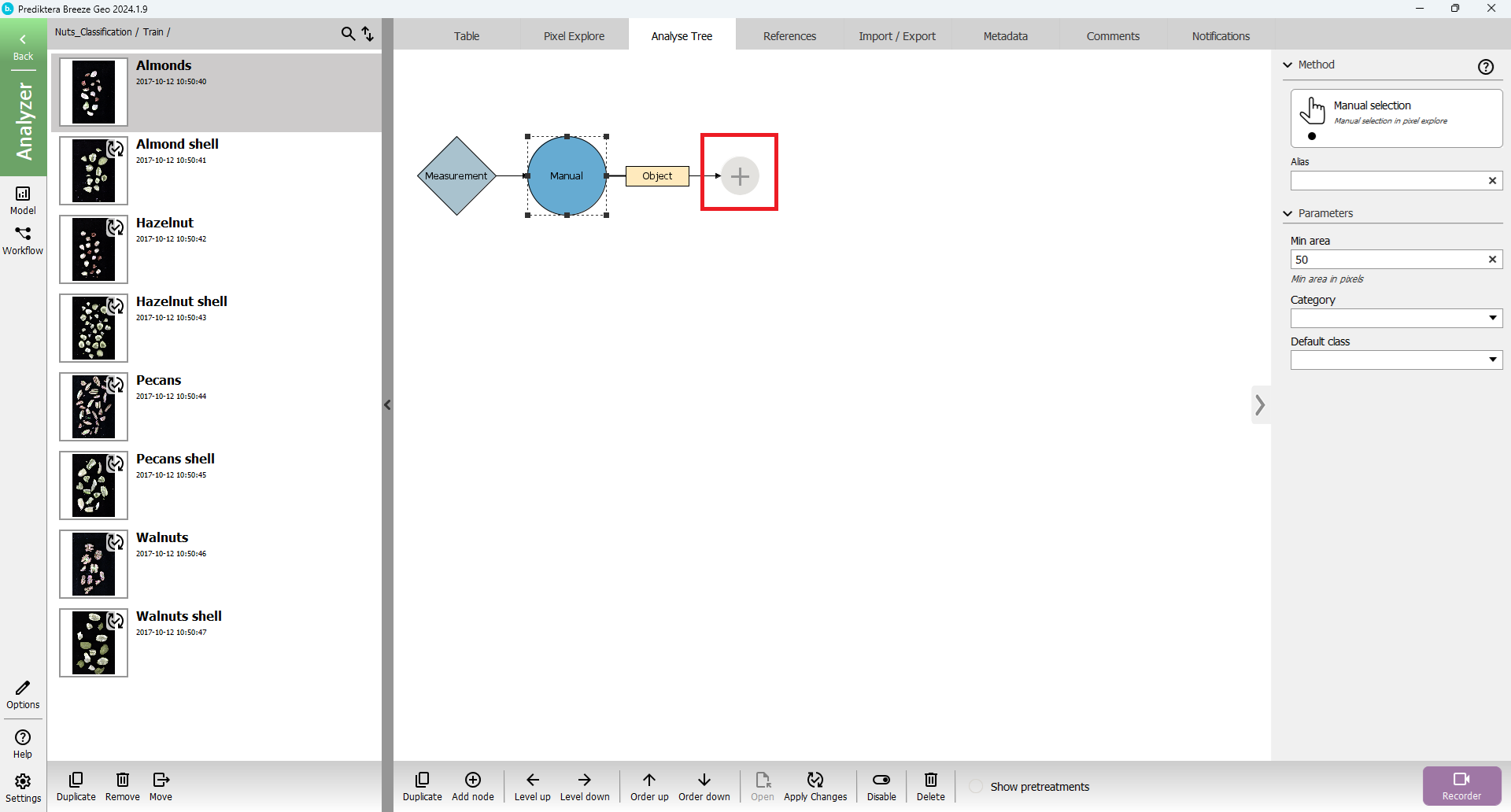
Klick “Up” until you are a the Studies level, then add a new node after the “Manual” segmentations node i the Analys Tree.

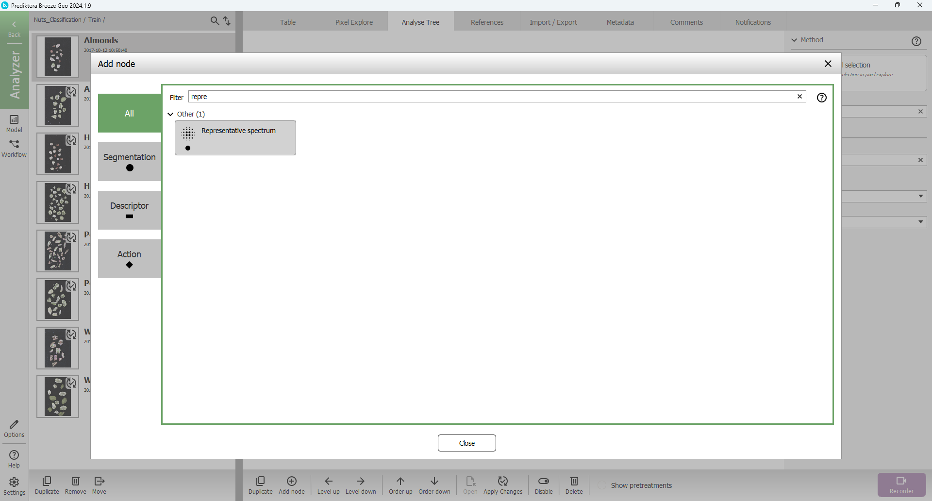
Browse or search for the Representative spectrum segmentation node:

Set some options on the “Representative spectrum” node:

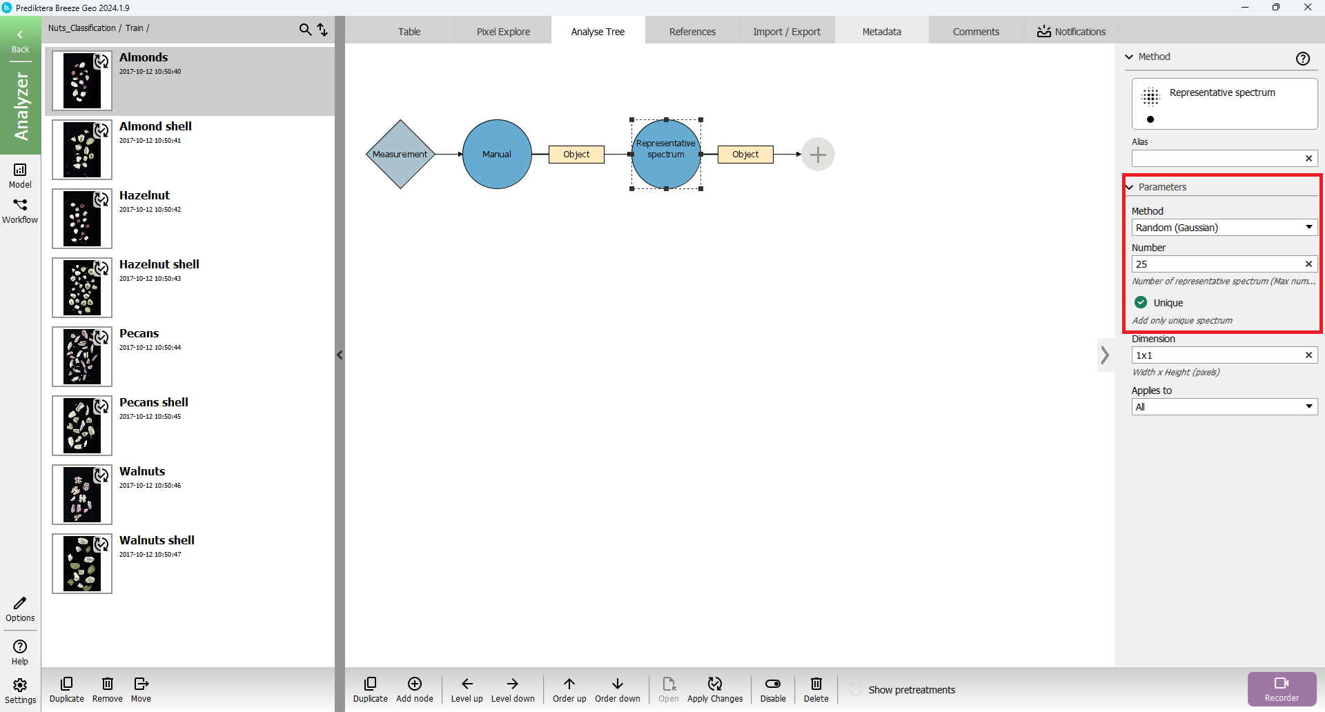
Press “Apply Changes” and Go to “Table” tab

Change Segmentation to “Representative Spectrum”

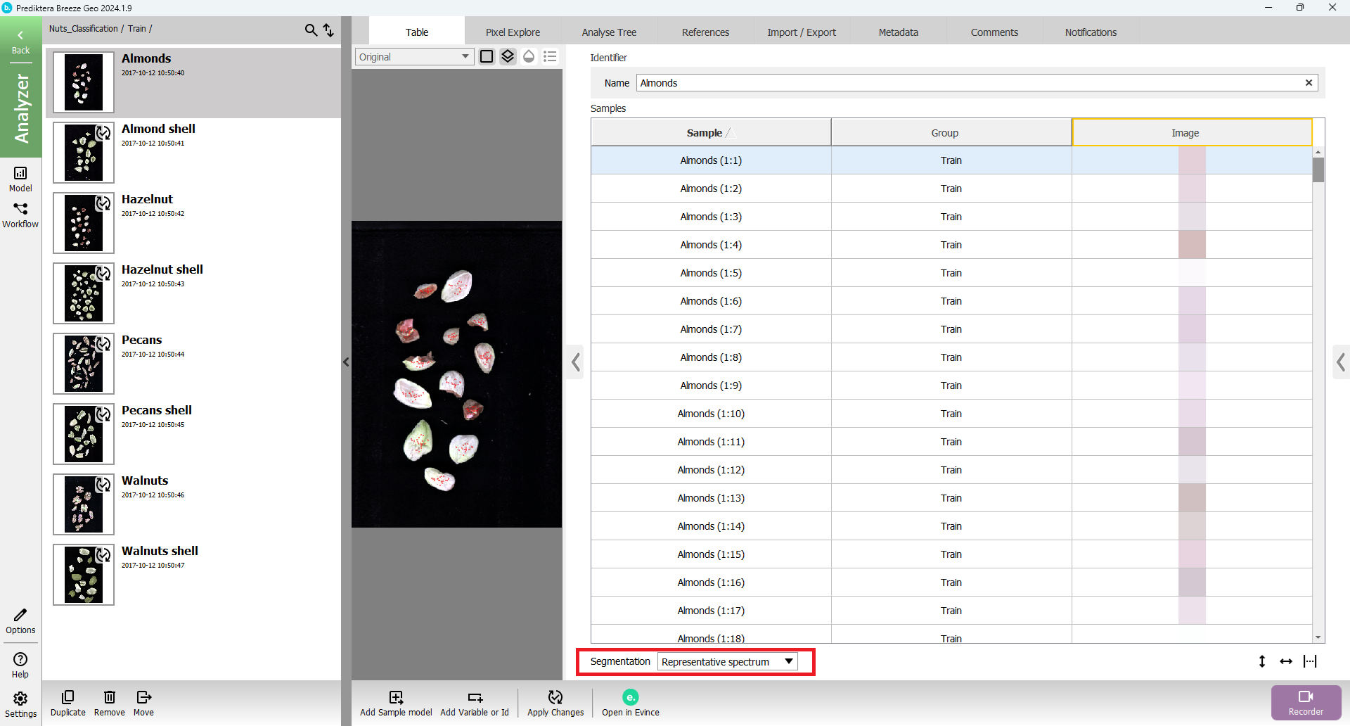
As you can see 25 pixels (i.e 25 spectra) have been selected from each sample.

Export segmentation

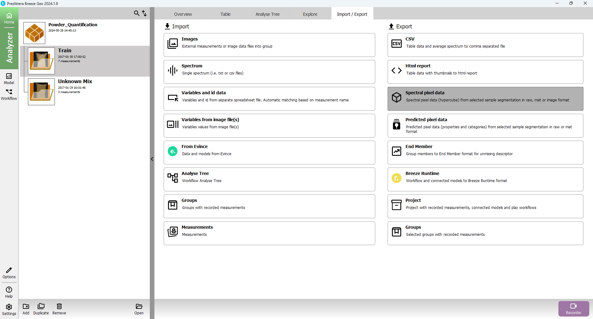
Press “Open” study to go to show groups (or dubble click on the study).

Select group to export, select “Export” tab, and select “Export spectral pixel data” (export the whole study by selecting the study instead of the group)
Press “Apply” button

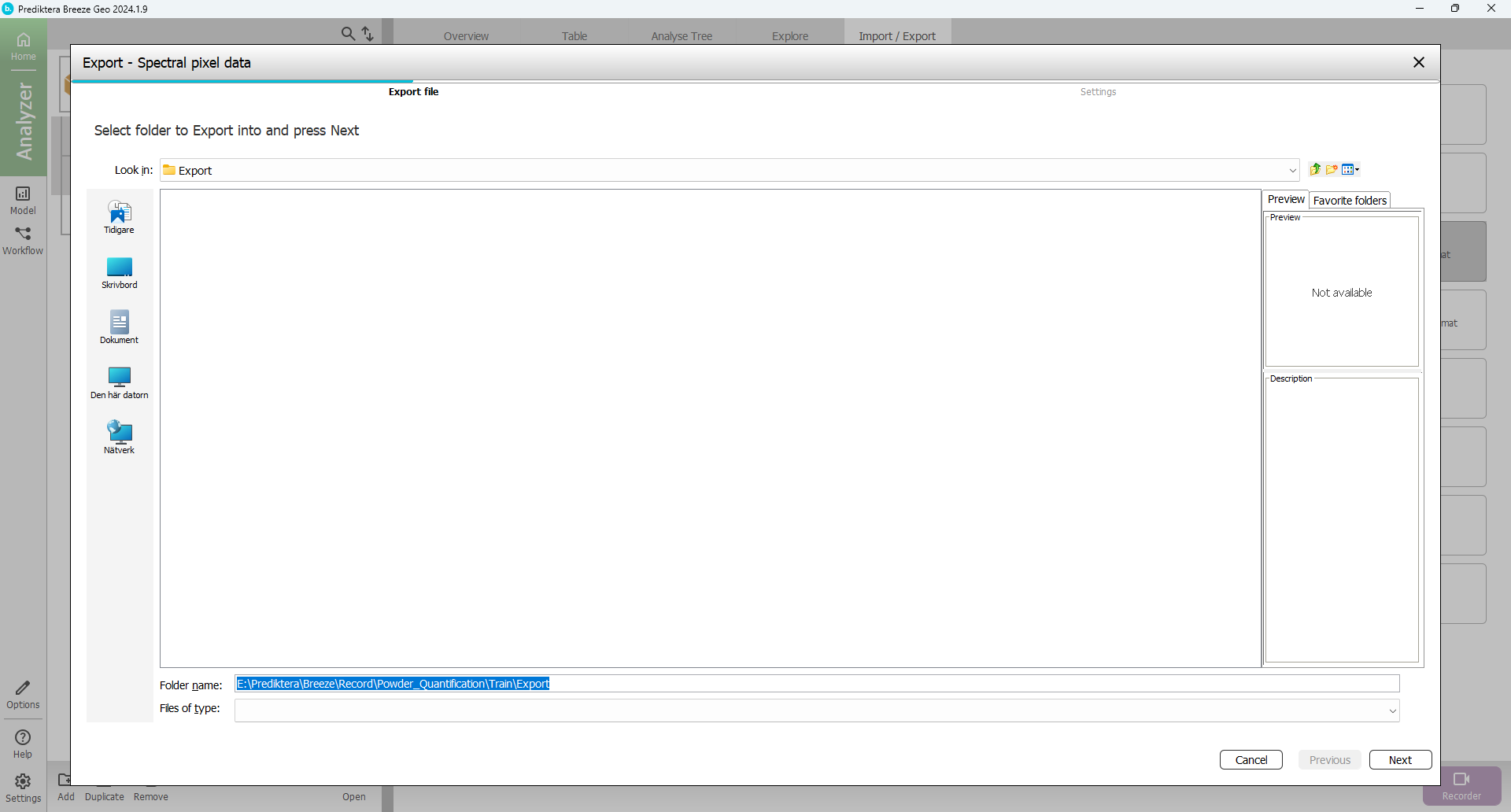
Select folder to Export to and press “Next”

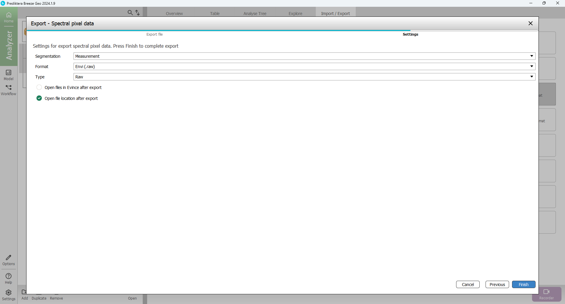
Choose segmentation to export

Choose “Format” (Raw or Matlab format)

Option: Select “Open files in Evince after export”

Requires that Evince is installed. You can also open the exported files in Evince manually.

Press “Finish”

The data is now segmented and exported to the selected folder

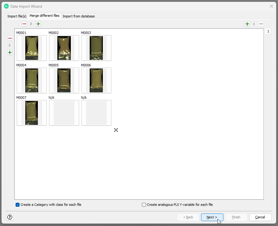
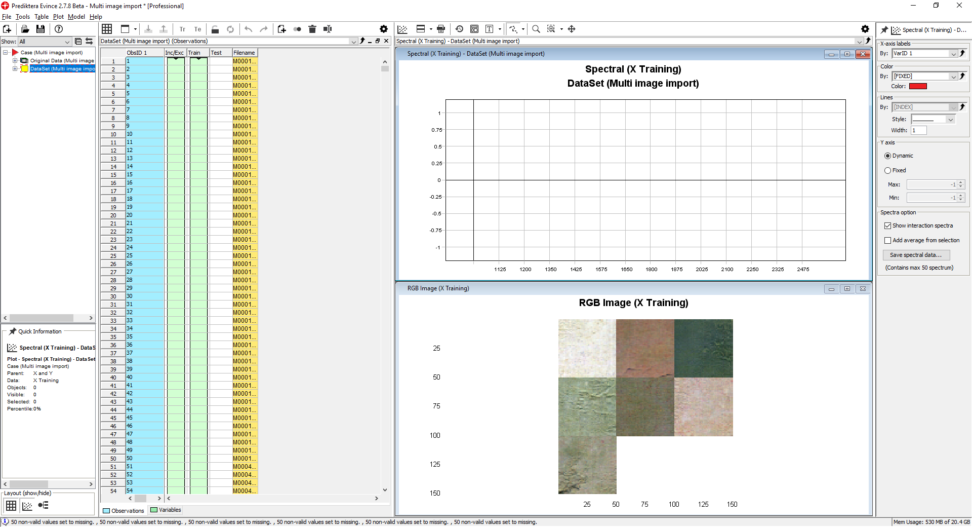
Finish the wizard and start working with the data in Evince

The Segmentation guide is now finished!

Feel free to test other segmentation options and play around with the Quantification of powder samples data.